Simplifying the Supplemental Security Income Program: Options for Eliminating the Counting of In-kind Support and Maintenance
Social Security Bulletin, Vol. 68, No. 4, 2008
The Supplemental Security Income (SSI) program's policies for both living arrangements and in-kind support and maintenance (ISM) are intended to direct program benefits toward persons with the least income and support, but they are considered cumbersome to administer and, in some cases, poorly targeted. Benefit restructuring would simplify the SSI program by replacing ISM-related benefit reductions with benefit reductions for recipients living with another adult. This article presents a microsimulation analysis of two benefit restructuring options, showing that the distributional outcomes under both options are inconsistent with a basic rationale of the SSI program.
Richard Balkus and Susan Wilschke are with the Office of Program Development and Research, Office of Retirement and Disability Policy (ORDP), Social Security Administration (SSA). Jim Sears is with the Division of Program Evaluation, Office of Research, Evaluation, and Statistics (ORES), ORDP, SSA. Bernard Wixon is with the Division of Economic Research, ORES, ORDP, SSA.
Acknowledgments: The authors are indebted to several individuals for their thoughtful comments: Paul Davies, Michael Leonesio, Linda Maxfield, Scott Muller, Kalman Rupp, Gloria Senden, and Paul Van de Water.
The findings and conclusions presented in the Bulletin are those of the authors and do not necessarily represent the views of the Social Security Administration.
Summary and Introduction
The Supplemental Security Income (SSI) program, administered by the Social Security Administration (SSA), is the income source of last resort for the low-income aged, blind, and disabled. As the nation's largest income-assistance program, it paid $38 billion in benefits in calendar year 2006 to roughly 7 million recipients per month. Because SSI is means tested, administering the program often requires month-to-month, recipient-by-recipient benefit recomputations. An increase in a recipient's income usually triggers a benefit recomputation. Or, an increase in the recipient's financial assets, which may render the recipient ineligible, would also prompt a recomputation. With this crush of ongoing recomputations, it is of little wonder that administrative simplification is a time-honored mantra for program administrators.
Against this backdrop, simplifying policy on food or shelter support to recipients from family and friends is especially compelling. Current policy on such in-kind support requires that recipients answer detailed questions about household composition, household expenses, and any contributions from the recipient and members of the household toward household expenses. This detailed household information is collected not only for initial applications, but also when there are changes in address, household composition, or household expenses. Moreover, although this information is collected for most recipients, much of it is unverifiable. Without question, these policies are well-intentioned because they target more means-tested benefits to recipients with no in-kind support. And, to be more equitable, there are separate computations for those who contribute significantly to household expenses and those who do not. Good intentions notwithstanding, there is a consensus among policymakers and program administrators that current SSI policies on in-kind support and maintenance (ISM) are complex, intrusive, and sometimes inequitable. In addition, these policies create a disincentive for families and friends who might otherwise increase food or shelter support to recipients. Finally, year-after-year ISM is shown to be a major source of payment error.
Over the years, policymakers have evaluated several alternatives to ISM in terms of (1) program costs; (2) distributional, poverty, and incentive effects; and (3) the degree to which they would actually simplify current policy. Of these alternatives, benefit restructuring has emerged as an interesting option because it simply eliminates all ISM-related benefit reductions, assuring program simplification. The benefit restructuring options considered here incorporate a cost neutrality constraint; that is, the cost of increasing benefits to recipients with ISM is fully offset by other benefit reductions. This study is a microsimulation analysis of the redistributional, poverty, and incentive effects of these benefit restructuring options.
Under benefit restructuring, benefit reductions for ISM recipients would be eliminated and, to offset the program cost increases, a smaller benefit reduction would be implemented for the large number of adult recipients who live with other adults. The rationale for these benefit reductions is that such recipients gain from economies of scale because of the shared costs of housing, food, and utilities. Administratively, the logic of benefit restructuring is that SSI should stop reducing benefits for ISM based on detailed tracking of income and contributions among family and friends. Instead, program administrators would determine the benefit size by simply establishing whether the recipient lives with another adult.
The study concludes that the two benefit restructuring options considered here would streamline current ISM policy by eliminating ISM-related benefit reductions, raising benefits for the 9 percent of recipients with ISM. Not only would benefit restructuring vastly simplify program administration, it would also encourage food and housing contributions to SSI recipients from family and friends. However, because of budget neutrality, we find that these options entail redistribution of $1.2 billion in annual benefits, affecting 50 percent to 75 percent of all recipients. In the end, this analysis brings to light a distributional concern affecting both options considered. Under the purest form of benefit restructuring, for example, those currently receiving ISM would have a benefit increase averaging $164 per month, funded through a benefit reduction averaging $44 per month for those who share housing. The distributional concern is that the initial per capita household incomes of those with benefit increases are, on average, 42 percent higher than the incomes of those with reductions, an outcome that is at odds with basic objectives of means-tested programs.
This article begins with an overview of the current benefit structure and rules for counting ISM, highlighting shortcomings and reviewing past simplification efforts. Next, we examine two benefit restructuring options, assessing how the options would simplify the program and discussing trade-offs, in terms of equity and incentive issues. We then provide a distributional analysis of recipients who would be better or worse off under either option. The article focuses on key subgroups of recipients, in terms of changes in SSI benefits and poverty status.
Current Policy: Description
Policies on living arrangements and ISM take into account the value of goods that some SSI recipients receive when living with others or from family or friends living outside the household. The Social Security Administration (SSA) uses a complex procedure to make ISM and living arrangement determinations for applicants when calculating the SSI benefit. There are two preliminary issues: (1) the living arrangement determination—whether SSI applicants are living in their own households or in the household of another adult, receiving food and shelter, and (2) the ISM determination—the type and amount of ISM, if any. In turn, these determinations affect the benefit computation. The full income guarantee, known as the federal benefit rate (FBR), is used for applicants living in their own households, while a reduced rate is used for those living in the household of another.1 In addition, if the full standard is used, the benefit is reduced if the applicant receives in-kind contributions of food or shelter.
Living Arrangement Categories
SSA uses four living arrangement categories to determine payment amounts. These categories are discussed in detail below.
Living Arrangement A. SSA first determines whether an adult, noninstitutionalized individual is living in his or her "own" household or living in the household of another. Living in one's "own" household means the person owns the home, has rental liability, or pays a pro rata share of household expenses. The benefit for such a person is based on 100 percent of the income guarantee. The great majority of recipients, 81 percent, are in living arrangement A (SSA 2007b, Table 5).
Living Arrangement B. This category is used when a recipient lives in the household of another and receives both food and shelter from other members of the household. This recipient is subject to a one-third reduction in the income guarantee. Almost 5 percent of SSI recipients are in living arrangement B.
Living Arrangement C. This is the category used for an eligible child younger than age 18 who lives with a parent. The benefit for such a recipient is based on 100 percent of the income guarantee. Twelve percent of SSI recipients are in living arrangement C. An eligible child is not charged with ISM for the food and shelter provided by the parent. The financial support provided by a parent is accounted for in the process called deeming.
Living Arrangement D. This category includes an eligible person living in a public or private medical institution, with Medicaid paying more than 50 percent of the cost of his or her care. This person is limited to an SSI payment of $30 per month. Only 2 percent of all SSI recipients are in this group. ISM is not countable for individuals who are in living arrangement D.
Two In-kind Support and Maintenance Rules
There are two ways ISM is counted. Both rules are used in conjunction with the living arrangement determination, but they have different effects on the benefit computation.
Value of the One-Third Reduction Rule (VTR). A recipient who lives in another person's household and receives both food and shelter from within the household (living arrangement B) has his or her income guarantee reduced by one-third. This reduction is taken in lieu of counting the actual value of the support that is received. However, a recipient who has some rental liability or pays at least a pro rata share of the household food and shelter costs would not be classified under living arrangement B and would not be subject to the VTR rule.
Presumed Maximum Value Rule (PMV). If an individual or a couple receives ISM but is not subject to the VTR rule, then the PMV rule applies. This rule would apply to an individual who lives in another person's household but does not receive both food and shelter from that person, or lives in his or her own household and receives in-kind support from either someone inside or outside of the household. The PMV equals one-third of the income guarantee plus $20 (the general income exclusion) and caps the amount of ISM that SSA counts. An amount less than the PMV may be used to calculate a person's payment if the individual can show that the actual value of the ISM received is lower than the PMV. Four percent of recipients are subject to the PMV. In 2006, 41 percent of recipients who received ISM under this rule were charged the maximum amount ($221 in 2006), while an additional 40 percent received ISM valued at $100 or less, and the remaining recipients were charged ISM ranging from $100 to the maximum amount. The PMV rule can require detailed documentation of contributions to the recipient and household expenses paid by all household members on an ongoing basis.
As shown in Table 1, 9 percent of recipients receive food or shelter support that result in a reduction in benefits. Roughly 5 percent of recipients live in the household of another (VTR) and a reduced income guarantee is used to calculate their benefits. For an additional 4 percent, the full income-guarantee level is used, but the benefits are reduced to offset contributions of food or shelter (PMV). Combining the two groups, roughly 6 percent of recipients receive substantial contributions that result in benefit reductions of one-third of the FBR, while the remaining 3 percent have smaller reductions. The elderly have slightly higher rates of ISM receipt than do other age categories.
| ISM type | Under 18 | 18–64 | 65 or older | All |
|---|---|---|---|---|
| VTR rule | 3.8 | 4.5 | 5.6 | 4.7 |
| PMV rule | 4.6 | 3.6 | 5.4 | 4.2 |
| Total | 8.4 | 8.0 | 11.0 | 8.9 |
| SOURCE: Social Security Administration, Supplemental Security Record (Characteristic Extract Record format), 100 percent data. | ||||
| NOTE: SSI = Supplemental Security Income; ISM = in-kind support and maintenance; VTR = value of the one-third reduction— recipients living in the household of another, receiving both food and shelter, and, hence, whose benefits are based on a federal benefit rate reduced by one-third; PMV = presumed maximum value—recipients receiving ISM, but not subject to the VTR rule. | ||||
Guaranteeing a Minimal Level of Support for SSI Recipients
The SSI benefit rate structure uses two income guarantees—an individual FBR ($637 per month in 2008) and a couple FBR ($956 per month in 2008), which is 150 percent of the individual level. In December 2006, 8 percent of recipients were members of eligible couples (SSA 2007b, Table 11). These income guarantees are adjusted for price changes annually.
The income guarantee can be thought of as the level of monthly income guaranteed to SSI recipients. That is, an individual recipient with no other income would receive $637 per month, and a recipient with income from other sources would receive a benefit equal to the difference between the income guarantee and his or her countable income. Income can exceed this level if income exclusions or state supplements are involved.2
As with ISM, assistance from other programs can also help a recipient meet his or her basic needs. Recipients may be eligible for other federally funded assistance such as food stamps and housing assistance. Forty percent of SSI recipients live in households that receive food stamps and 9 percent receive housing assistance (SSA 2008, Table 7). Of those recipients who live with another adult and, therefore, would be affected by this policy change (both those experiencing an increase or a decrease in benefits), roughly one-quarter live in households that receive food stamps.3
Although the FBR does not guarantee poverty-level income, nonetheless, many SSI recipients live in households with income exceeding the poverty threshold.4 An SSI recipient may not have access to the income of other household members, but may benefit from living in a household that can afford to spend more on food and shelter. By contrast, income from a parent (in the case of a minor child) or an ineligible spouse is counted as income to that recipient, less certain exclusions. Furthermore, any cash support provided by other household members is counted as income to the SSI recipient and the SSI benefit is reduced accordingly.
Despite the benefit reductions that are based on living arrangements and ISM, wide disparities remain in household income between subgroups of SSI recipients. Table 2 shows that adult recipients living with another adult have the lowest rates of household poverty (24 percent), compared with a 90 percent poverty rate for adults who live alone or only with minor children. As this analysis will later explain, among those recipients who live with others, there are differences in poverty rates and levels of household income between those who currently receive ISM and those who do not.
| Living arrangement/age category | Recipient distribution | Household income as a percentage of the poverty threshold | |||
|---|---|---|---|---|---|
| Under 100 (poor) | 101 to 200 | 201 to 300 | Over 300 | ||
| Adult with eligible spouse | 9 | 52 | 36 | 4 | 8 |
| Adult with another adult a | 49 | 24 | 44 | 15 | 16 |
| Adult without another adult | 27 | 90 | 10 | 0 | 0 |
| Child recipient | 15 | 43 | 41 | 12 | 5 |
| SOURCE: Social Security Administration's Financial Eligibility Model. | |||||
| NOTES: SSI = Supplemental Security Income. | |||||
| a. Includes adult recipients living with either nonspouse adults or ineligible spouses. | |||||
Differences in household poverty levels are not surprising because SSI makes payments to individuals or couples, whereas household poverty measures take into account income of other household members. SSI benefit calculations are based primarily on the income of the individual or couple, but deeming and ISM/living arrangement policies are used to adjust for support from other household members or, for that matter, from family and friends who live outside the household. This focus on the individual, as well as the counting of in-kind income, distinguishes the SSI program from many means-tested programs. Most other means-tested programs, in the United States and elsewhere, do not count in-kind income when determining eligibility and benefit amounts. The Food Stamp Program (FSP), Temporary Assistance for Needy Families (TANF), and needs-based programs in countries such as Canada and Australia, for example, exclude in-kind income from eligibility and benefit calculations. The FSP and TANF, however, pay benefits to a household based on the income of all household members, with some exclusions. The FSP compares household income with federal poverty guidelines in determining eligibility.
Current Policy: Administrative, Incentive, and Equity Issues
The state programs that preceded SSI often undertook detailed analysis of the household budget to establish an applicant's level of financial need. One of the founding principles of SSI is that, as a program that is national in scope, it should be based on a "flat grant" approach that does not involve program administrators in the detailed household budgets of millions of recipients. The law creating the SSI program included the one-third reduction provision so that SSA would not have to determine the actual value of room and board when a recipient lived with a friend or relative. A congressional committee report5 indicated that the reduction would apply regardless of whether the individual made any payment toward household expenses. Although the provision was intended to be simple to administer, it did not adequately address differences in living arrangements among SSI recipients. SSA created the PMV rule and the pro rata-share concept through regulations in an attempt to better address equity among recipients. However, these regulations compromised the simplification objective of the "flat grant" approach: "Over the life of the program, those policies have become increasingly complex as a result of new legislation, court decisions, and SSA's own efforts to achieve benefit equity for all recipients" (Government Accountability Office (GAO) 2002). This section illustrates some of the trade-offs that policymakers face when seeking to simplify complex program rules.
Administrative Complexity
Although only 9 percent of recipients receive ISM, SSA must determine the appropriate living arrangement category for all recipients and must determine receipt of ISM for most recipients. In some cases, the determination is straightforward, such as establishing whether a recipient owns a home. For other cases, a determination may involve a detailed accounting of household expenses and the individual's contribution, to establish whether the individual pays his or her pro rata share of expenses. In addition to initial claims, this determination must be repeated if there is any change in household composition or expenses that might affect the amount of the SSI benefit.
ISM and living arrangements often cause payment errors because recipients frequently do not understand or comply with reporting requirements. According to the fiscal year 2006 SSI Payment Accuracy Report (SSA 2007a), living arrangements and ISM have been among the major causes of overpayment and underpayment deficiency dollars in recent years. For example, in 2006 living arrangements and ISM accounted for $494 million in overpayment deficiency dollars and $339 million in underpayment deficiency dollars.
Although SSI eligibility was intended to be determined on the basis of objective information on income and resources, development of ISM is often based on estimates of food and shelter expenses provided by the applicant or recipient and verified by other household members. As stated by the Social Security Advisory Board, "The [living arrangements/in-kind support] process is weak because most allegations…(such as household expenses, rental subsidy, separate purchase of food, sharing, etc.) are verified using a corroborative statement from someone known to the applicant and who may have a motivation to be less than objective and truthful. There is no practical way to verify these issues" (SSA 2005, 9).
Despite specific instructions for developing ISM, the same level of contribution could result in different payment amounts, depending on how it is allocated. Consider, for example, a recipient who lives with three others and contributes $300 per month toward household expenses. The monthly housing expenses are $1,200 and the food expenses are $500. If the recipient's contribution was allocated toward overall household expenses, it would fall short of his or her pro rata share ($425) and the recipient would be considered to be in living arrangement B, with a one-third reduction ($212) in the FBR. However, under current program rules, the recipient could earmark his or her contribution specifically for shelter expenses. In that case, the recipient is meeting his or her pro rata share of shelter expenses and would be assigned to living arrangement A. The recipient would be charged for the ISM he or she receives as food, and the SSI benefit would be reduced by $125, his or her pro rata share of food. Hence some recipients avoid benefit reductions by earmarking contributions. By implication, such recipients hold an arbitrary, unfair advantage over uninformed recipients with similar financial resources, by virtue of information received from program administrators or advocacy groups.
Similarly, ISM policies have complicated the administration of the Medicare Modernization Act of 2003. This act established a low-income subsidy program for drug premiums and co-payments. Although the program generally follows the SSI definition of income and resources, it used higher income and resource limits and a simpler approach to defining ISM. However, despite this attempt to streamline the Medicare low-income subsidy process, criticism of the use of ISM in the low-income subsidy process persisted. With the Medicare Improvement for Patients and Providers Act of 2008 (Public Law 110-275), Congress voted to exclude in-kind support and maintenance from income when determining eligibility for the low-income subsidy program.
Equity and Incentive Issues
In some cases, policies on living arrangements and ISM promote equitable treatment among SSI recipients by reducing benefits for those individuals who receive support from others. SSI recipients who receive ISM may live with others who have income levels that allow the household to spend more on food and shelter than is the case for SSI recipients in other household situations. Consider the example of a disabled adult living with his or her parents and contributing $300 toward the household expenses. The parents' combined monthly income of $4,000 allows them to spend about $2,100 a month on food and shelter expenses. The parents' income is not considered in determining the amount of the SSI benefit for their disabled adult child. However, the disabled adult child gains from living in a household that spends more on food and shelter expenses ($700 per household member) than what could be spent relying solely on his or her SSI benefit. Because this person's $300 payment is less than the prescribed pro rata share, he or she is considered "living in the household of another" and subject to the one-third reduction. Hence, SSI policies accurately target benefit reductions to some recipients living in households that are better off than others.
However, ISM rules do not always result in equal treatment among recipients. The policies also allow some recipients to live in households that are better off than others and not be charged ISM. Consider the same example with one change. The parents have paid off their mortgage, reducing their monthly household expenses to $900. The disabled adult child's monthly payment now equals his or her pro rata share. Therefore, he or she is no longer subject to the one-third reduction. The outcome is higher monthly household income with lower household expenses—a result one would not expect from a means-tested program.
The incentives created by living arrangement and ISM policies are another area of concern. ISM policies may discourage friends and family from making contributions of food and shelter to SSI recipients because such contributions are offset by dollar-for-dollar reductions in the recipient's benefits, up to $232 (the presumed maximum value, or equivalently one-third of the income guarantee plus $20).6 There are no further benefit reductions after contributions reach one-third of the income guarantee. This creates a substantial disincentive to contribute a modest amount (less than $232) and no disincentive at all for contributions above $232. A family making a $200 rent payment for a family member receiving SSI will see a dollar-for-dollar reduction in the SSI recipient's monthly benefit. In practical terms, after the benefit reduction, the recipient would be no better off. On the other hand, a family able to afford a monthly rent contribution of $800 would induce a benefit reduction of $232, so the standard of living of the SSI recipient would be substantially improved. By capping the amount of contributions that are counted, some recipients receiving large amounts of ISM receive the same benefits as recipients who receive smaller amounts of ISM, which seems inequitable.
Why are there such disincentives in the SSI program? From one perspective, current SSI policy simply treats in-kind income just as it does income from other sources. Unearned income results in a dollar-for-dollar reduction in the SSI benefit. However, policymakers may wish to encourage contributions to SSI recipients, just as current policies are designed to encourage earnings.
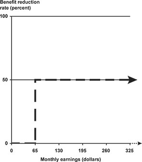
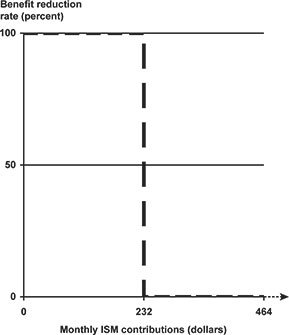
Charts 1 and 2 compare treatment of ISM with treatment of earnings in calculating SSI benefits. Chart 1 shows how SSI benefits are reduced for different levels of monthly earnings. The first $65 of earnings does not result in any benefit reduction, encouraging recipients to enter the labor force.7 At higher levels of earnings, benefits are reduced $1 for each $2 of earnings. Recipients are able to raise their standards of living by working and continuing to receive some SSI benefits until monthly earnings reach $1,359. In contrast, current ISM policy imposes a dollar-for-dollar (100 percent) benefit reduction for all contributions less than $232 per month and no reduction for support above that level (see Chart 2). Under SSI earnings policies, low earners enjoy the effects of the earnings disregards, and under ISM, it is recipients whose families make large contributions (over $232 per month) who benefit from an ISM disregard. Although current ISM policies have several rationales, little attention has been given to formulating policies that actually encourage contributions to SSI recipients by their families and friends.
Treatment of earnings under SSI
Text description fo Chart 1.
Treatment of earnings under SSI
Chart 1 is a line chart that illustrates the rate at which SSI benefits are reduced according to recipient earnings.
The vertical axis is labeled "benefit reduction rate (percent)." Zero, 50, and 100 percent intervals are marked on the axis. The horizontal axis is labeled "monthly earnings (dollars)." Dollar amounts from zero to 325 are marked on the axis in 65-dollar increments.
A line showing the benefit reduction rate starts at the zero-zero coordinate and remains flat at the zero-percent level moving left to right until it reaches 65 dollars. At that point the line turns 90 degrees and moves directly upward until it reaches the 50 percent level. Then the line again turns 90 degrees and moves left to right at the 50 percent level where it remains beyond the 325-dollar mark.
Treatment of ISM contributions under SSI
Text description for Chart 2.
Treatment of ISM contributions under SSI
Chart 2 is a line chart that illustrates the rate at which SSI benefits are reduced according to in-kind support and maintenance (ISM) contributions.
The vertical axis is labeled "benefit reduction rate (percent)." Zero, 50, and 100 percent intervals are marked on the axis. The horizontal axis is labeled "monthly earnings (dollars)." Zero, 232, and 464 dollar amounts are marked on the axis.
A line showing the benefit reduction rate starts at the zero dollars-100 percent coordinate and remains flat at the 100-percent level moving left to right until it reaches 232 dollars. At that point the line turns 90 degrees and moves directly downward until it reaches the zero percent level. Then the line again turns 90 degrees and moves left to right at the zero percent level where it remains beyond the 464-dollar mark.
In contrast to assistance from family and friends, certain government or charitable assistance is not counted as income. For example, while a rent subsidy provided by a family member is counted as ISM and reduces the SSI benefit, government-funded housing subsidies are excluded by law. This discourages family members from helping and encourages reliance on government programs. In addition, the one-third reduction might deter some recipients from living with others because it results in reduced benefits. Some recipients may choose less than optimal living situations in order to receive higher benefits.
With many strikes against it, how have current ISM/living arrangement policies managed to survive? First, the estimated program costs of eliminating ISM-related benefit reductions would total roughly $1.2 billion annually.8 Second, the distributional impact of counting ISM is consistent with the goals of the program; that is, current policies demonstrably target benefit reductions to recipients who live in higher-income households and who receive support—sometimes substantial support—from family and friends. Efforts to simplify current policy must be viewed against this backdrop.
The question for policymakers is whether the administrative complexity required to make ISM/living arrangement determinations is justified or whether there is a better way to adjust for differences in household situations and support for SSI recipients. The challenge is to target benefits to those individuals with the greatest need, but to do so in a way that can be administered fairly, efficiently, and without an increase in program costs.
Past Simplification Efforts
Since the inception of the SSI program in 1974, at least 10 workgroups, studies, and reports have focused on simplifying SSI policies. Most of these efforts contained options or recommendations for simplifying living arrangements and ISM (SSA 2000). Despite the sustained focus on this policy area, limited progress has been made toward simplifying these rules. Recent actions include a change in regulations that removed clothing from the definition of in-kind support and maintenance so that recipients are no longer required to report gifts of clothing.9
Since GAO's designation of SSI as a high-risk program in 1997 (a designation removed by GAO in 2003), benefit restructuring has received more attention than any other approach for simplifying living arrangement and ISM rules. SSA's SSI Legislation Workgroup that was convened in 1997 to provide legislative options for reducing payment errors analyzed this approach and identified several options for benefit restructuring in its final report.
SSA's former Office of Policy (currently the Office of Retirement and Disability Policy) in its December 2000 report, Simplifying the Supplemental Security Income Program: Challenges and Opportunities (SSA 2000), further analyzed benefit restructuring as one option for simplifying living arrangement and ISM policies. While noting the potential for program simplification, the report expressed concern about the effect that benefit restructuring would have on the program objectives of benefit equity and benefit adequacy. It emphasized the need to further assess the options and the trade-offs between maximizing the underlying objectives of the program and simplifying the program.
GAO (2002) acknowledged SSA's 2000 report on SSI program simplification and recommended that SSA "identify and move forward in implementing cost-effective options simplifying complex living arrangements and in-kind support and maintenance policies, with particular attention to those policies most vulnerable to fraud, waste, and abuse." SSA concurred with the recommendation and also stated in its SSI Corrective Action Plan that it would further analyze the distributional effects of options for simplifying living arrangement and ISM policies.
ISM Elimination Options: Description
Two policy options are simulated in this analysis. Both options implement budget neutrality by reducing federal income-guarantee levels for adult SSI recipients living with other adults, offsetting the cost of benefit increases to current recipients with ISM:
The 7/0 option reduces the FBR by 7 percent for adults. It does not change the FBR for child recipients, nor does it change the FBR for adult recipients with no other adults in the household.The 10/5 option reduces the FBR by 10 percent for adults, with no reduction for child recipients. However, this option does include a 5 percent FBR increase for adult recipients with no other adults in the household—a subgroup with a poverty rate of 90 percent.
Under these policy options, in-kind support would no longer be counted in determining eligibility or the monthly benefit amount, resulting in benefit increases for those receiving ISM. The budgetary logic of benefit restructuring is that the substantial benefit reductions associated with ISM would end, and instead, a smaller benefit reduction would be assessed to each of the large number of recipients—about half of all recipients—who live with other adults.10 The two benefit restructuring options considered here have been modeled with a budget neutrality constraint. That is, program cost increases associated with eliminating ISM are offset by savings—in this case, benefit reductions—of equal value. These reductions do not represent the amount recipients save by sharing housing, but rather reflect the program savings required to offset the cost of eliminating ISM. Cost estimates generated as a byproduct of our simulation analysis have shown that each of the two options is approximately budget neutral.11
ISM Elimination Options: Administrative, Incentive, and Equity Issues
The options described here would simplify the administration of the SSI program. However, as discussed below, they involve other trade-offs.
Administrative Complexity
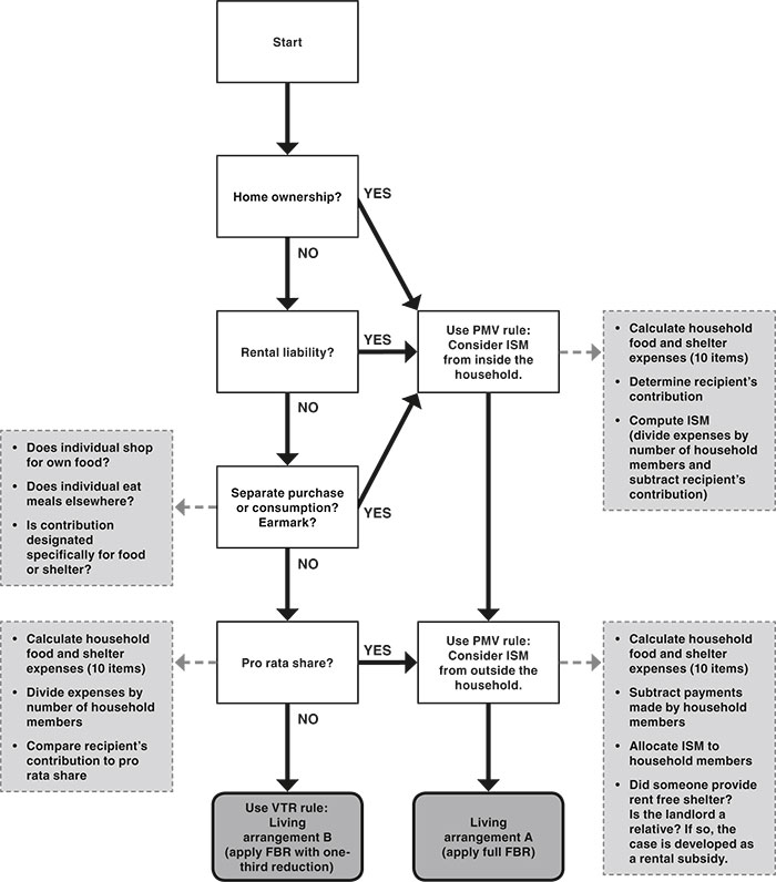
Chart 3 is a simplified flow chart of the current living arrangement and ISM process that illustrates the complexity of the process, especially at certain steps.12 In the most complex cases, the process involves a detailed accounting of household expenses and the individual's contribution, to determine whether the individual pays his or her pro rata share of expenses.
Simplified illustration of current SSI living arrangement and ISM process
Text description for Chart 3.
Simplified illustration of current SSI living arrangement and ISM process
Chart 3 is a flow chart showing the following.
If home ownership or rental liability equals yes then use the presumed maximum value rule: Consider ISM from inside the household:
- Calculate household food and shelter expenses (10 items)
- Determine recipient's contribution
- Compute ISM (divide expenses by number of household members and subtract recipient's contribution
then apply the full federal benefit rate (FBR) for living arrangement A.
If home ownership or rental liability equals no then evaluate separate purchase or consumption:
- Does individual shop for own food?
- Does individual eat meals elsewhere?
- Is contribution designated specifically for food or shelter?
if yes:
- Calculate household food and shelter expenses (10 items)
- Determine recipient's contribution
- Compute ISM (divide expenses by number of household members and subtract recipient's contribution
then apply the full federal benefit rate (FBR) for living arrangement A.
If home ownership, rental liability, and separate purchase for consumption equal no then evaluate the pro rata share:
- Calculate household food and shelter expenses (10 items)
- Divide expenses by number of household members
- Compare recipient's contribution to pro rata share
if yes, use PMV rule: Consider ISM from outside the household:
- Calculate household food and shelter expenses (10 items)
- Subtract payments made by household members
- Allocate ISM to household members
- Did someone provide rent free shelter? Is the landlord a relative? If so, the case is developed as a rental subsidy.
then apply the full federal benefit rate (FBR) for living arrangement A.
If home ownership, rental liability, separate purchase or consumption, and pro rata share equal no then use the Value of the One-Third Reduction Rule: living arrangement B and apply the FBR with a one-third reduction.
With benefit restructuring, SSA would not be concerned with the amount of household expenses, the recipient's contributions to those expenses, or how they are paid. These options reflect an approach that is much simpler administratively. Living arrangement development would be limited to determining whether the recipient lives with an adult, as shown in Chart 4. SSA estimates that the administrative savings from option 7/0—totally eliminating ISM—would be $70 million annually, after start-up costs associated with the first year of implementation.13
SSI living arrangement development process under benefit restructuring
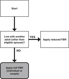
Under benefit restructuring, SSA would continue to rely on recipients to report certain living arrangement changes, but only whether the recipient began or stopped living with an adult. Certainly, payment accuracy would improve because program administrators would no longer have to track changes in household expenses and contributions, nor would they need to process the array of allegations and confirmations underlying the information currently collected on expenses and contributions.
Equity and Incentive Issues
Under the options considered here, contributions of food or shelter would no longer be tracked or measured by SSA, nor would recipients receiving such assistance have their benefits reduced. In-kind contributions of any amount would be encouraged because benefit reductions would no longer be assessed to those receiving contributions of shelter, utilities, or food. Encouraging in-kind support seems consistent not only with recent efforts to augment benefits from public programs with private or charitable contributions, but also with long-term efforts to increase the level of well-being of as many recipients as possible.
However, one further implication of such a policy should be noted. The objective of SSI policy is generally to bring the incomes of SSI recipients to the approximate level of the income-guarantee level. This is mostly true, even though some recipients have higher incomes as a result of provisions such as state supplements, income exclusions, and the exclusion of ISM above the current limit. The policies considered here, by removing the benefit reductions assessed to recipients with ISM, would permit and encourage higher levels of economic well-being for some SSI recipients—those receiving support in the form of food or shelter. If one assumes that all SSI recipients should enjoy a similar level of economic well-being, this may seem inequitable. However, one implication of encouraging in-kind support is that the income guarantee would increasingly represent a minimum income level, rather than a uniform income level. And, among those with higher levels of economic well-being would be not only recipients with earnings, state supplements, or their own homes, but also those receiving in-kind contributions.14
Depending on the size of the benefit reductions adopted, the options may also discourage recipients from sharing housing. Under current policies, benefit reductions that are due to ISM may discourage shared housing, especially for recipients who might be subject to a one-third reduction in the FBR if they cannot pay their pro rata share of expenses. However, most recipients who live with other adults do not have their benefits reduced. But under the policy options considered here, such recipients would experience either a 7 percent or a 10 percent reduction in the income-guarantee level used to compute their benefits. In addition, under the 10/5 option, the income-guarantee level used to compute benefits for recipients living alone would be increased by 5 percent. The net result is that option 10/5 would create a gap of roughly 17 percent between the income-guarantee level for recipients living alone and those living with other adults. Such a difference in income guarantees and resulting benefits may represent a disincentive to share housing for roughly half of all SSI recipients.
ISM Elimination Options: Simulated Effects
This section describes the distributional and poverty effects of benefit restructuring on SSI recipients.
Simulation Methodology
The simulation results are derived from the Financial Eligibility Model (FEM)—a static SSI simulation model developed by SSA's Office of Research, Evaluation, and Statistics staff—which has been substantially enhanced in order to analyze benefit restructuring options. The FEM includes a detailed SSI benefit calculator, as well as behavioral modules that estimate whether individuals exit or enter the SSI rolls, based on the policy options simulated. The FEM is based on the Survey of Income and Program Participation (SIPP), exact matched to SSA administrative records using Social Security numbers (SSNs) reported by survey respondents. The survey estimates reflect the noninstitutional population of the United States, and all data represent the reference month of November 1996, but dollar estimates have been price-adjusted to 2008. The Supplemental Security Record data are the source of information on current-pay status and monthly federal benefits for participants, as well as other programmatic characteristics of participants, such as receipt of ISM. See the appendix for more detailed information on the simulation methodology.
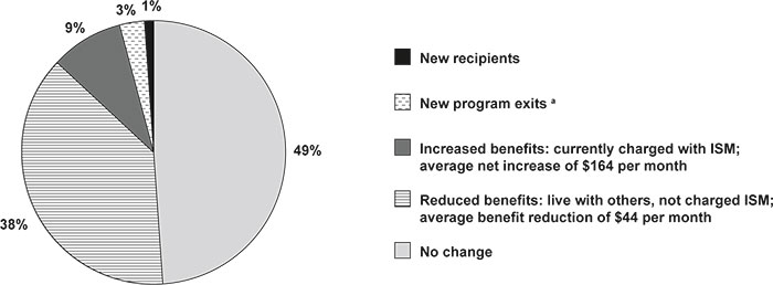
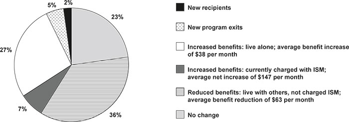
Summary Effects. Charts 5 and 6 present summary results for the two simulations. Chart 5 illustrates the basic distributional features of benefit restructuring. We see that 9 percent of beneficiaries have benefit increases under option 7/0. The majority of these recipients live with other adults and would also be subject to the 7 percent reduction, although the effect on their monthly SSI benefits would be a net increase. A subset of that group would receive their increases from the elimination of ISM and would not be subject to any benefit reductions because they either live alone, they live only with minor children, or they are members of an eligible couple. The benefit increases for this entire group would be substantial—on average the monthly increase in benefits would be $164, a 44 percent increase. Under option 10/5, current ISM recipients would also experience substantial benefit increases, averaging $147 per month, but, in addition, there would be a second recipient subgroup with increases in benefits. By design, option 10/5 provides benefit increases to the 27 percent of recipients who live alone or with minor children. Their benefits would increase by $38 per month, on average. In all, 34 percent of recipients would have benefit increases under option 10/5.
Percentage distribution of SSI recipients under option 7/0
| Distribution of SSI recipients | Percent |
|---|---|
| New recipients | 1 |
| New program exits a | 3 |
| Increased benefits: currently charged with ISM; average net increase of $164 per month | 9 |
| Reduced benefits: live with others, not charged ISM; average benefit reduction of $44 per month | 38 |
| No change | 49 |
Percentage distribution of SSI recipients under option 10/5
| Distribution of SSI recipients | Percent |
|---|---|
| New recipients | 2 |
| New program exits a | 5 |
| Increased benefits: live alone; average benefit increase of $38 per month | 27 |
| Increased benefits: currently charged with ISM; average net increase of $147 per month | 7 |
| Reduced benefits: live with others, not charged ISM; average benefit reduction of $63 per month | 36 |
| No change | 23 |
For both policy options, the costs of benefit increases to the 8 percent to 9 percent of recipients with ISM are recovered through smaller reductions to about half of all recipients—those who share housing.15 Under 10/5, the benefit reductions assessed to those in shared housing are larger, covering the additional cost of benefit increases to recipients living alone.
Under each option, about half of all SSI recipients are assessed benefit reductions, although roughly 9 percent also would have larger, offsetting benefit increases because of the elimination of ISM provisions. The residual group—about 41 percent of all recipients—would have net reductions in their monthly benefits, including those leaving the rolls (see Charts 5 and 6). This group is comprised mainly of those who live with other adults, but are not currently receiving ISM. Under 7/0, the average reduction would be $44 per month for those living with others, and under 10/5 it would be $63 per month. The simulations show a net reduction in SSI recipients of 2 percent under each option.
The two policy options are broad in scope. In all, over 50 percent of recipients would have benefit changes under 7/0, and over 75 percent of recipients would have benefit changes under 10/5.
Subgroup Effects. The key subgroups include those whose benefits increase or whose benefits are reduced under the two options. We begin by considering option 7/0.
Under 7/0, there are two key subgroups: (1) 9 percent of recipients receiving ISM under current law would have benefit increases that are often sizable, and (2) 41 percent of recipients who are living in shared housing would have benefit reductions (see Chart 5). The latter subgroup is composed of those who we estimate would exit the SSI rolls (3 percent) and those we estimate to have benefit reductions but who would continue to receive benefits (38 percent).16
Let us consider the demographic and household characteristics of these two groups, as shown in Table 3, columns 2 and 3. Column 2 includes those with net benefit increases under 7/0. Most recipients with net benefit increases live with other adults and, hence, would be assessed the 7 percent FBR reductions; however their ISM-related benefit increases would be larger, yielding net increases. Ten percent of both the aged and disabled adults have net benefit increases (see Table 3, column 2). Male recipients, white non-Hispanics, and Hispanic/other recipients are somewhat more likely to have ISM and, consequently, net benefit increases.
| Recipient characteristic | Presimulation recipient distribution (1) | ISM elimination options | |||
|---|---|---|---|---|---|
| 7/0 | 10/5 | ||||
| Those with increases (2) | Those with reductions (3) | Those with increases (4) | Those with reductions (5) | ||
| Percentage with benefit changes a | |||||
| Living arrangements | |||||
| Adult with eligible spouse | 10 | 0 | 0 | b | 0 |
| Adult without another adult | 32 | 4 | 0 | 96 | 0 |
| Adult with another adult c | 58 | 14 | 82 | 14 | 82 |
| Aged/disabled adults | |||||
| Aged | 32 | 10 | 32 | 48 | 31 |
| Disabled adults | 68 | 10 | 54 | 38 | 52 |
| Sex | |||||
| Men | 42 | 12 | 52 | 34 | 40 |
| Women | 58 | 9 | 43 | 46 | 37 |
| Race/ethnicity | |||||
| White non-Hispanic | 49 | 11 | 42 | 44 | 41 |
| Black non-Hispanic | 29 | 8 | 52 | 43 | 50 |
| Hispanic and other | 22 | 11 | 49 | 34 | 48 |
| Changes in monthly SSI benefits d (average $) | |||||
| All adult recipients | … | 164 | -44 | 63 | -63 |
| Adult with eligible spouse | … | … | … | … | … |
| Adult without another adult | … | 149 | … | 38 | … |
| Adult with another adult c | … | 165 | -44 | 147 | -63 |
| Average percentage change | |||||
| All adult recipients | … | 44 | -9 | 16 | -13 |
| Adult with eligible spouse | … | … | … | … | … |
| Adult without another adult | … | 43 | … | 9 | … |
| Adult with another adult c | … | 44 | -9 | 39 | -13 |
| Income measures | |||||
| Median monthly per capita household income ($) | … | 937 | 659 | 693 | 653 |
| Median monthly per capita family income ($) | … | 859 | 632 | 693 | 615 |
| Presimulation rate for households (%) | … | 27 | 27 | 75 | 26 |
| Postsimulation rate for households (%) | … | 24 | 29 | 72 | 31 |
| SOURCE: Social Security Administration's Financial Eligibility Model. | |||||
| NOTES: SSI = Supplemental Security Income; ISM = in-kind support and maintenance; CPI = Consumer Price Index; … = not applicable. | |||||
| a. The estimates are as a percentage of all recipients in each group. The table is based on persons receiving SSI. Estimates are based on adult recipients only. Although 5 percent of child recipients have a benefit increase under 7/0, by design benefit reductions are limited to adult recipients. | |||||
| b. Insufficient sample size. | |||||
| c. Includes adult recipients living with either a nonspouse adult or an ineligible spouse. | |||||
| d. The income and benefit estimates have been CPI-adjusted to represent 2008. The income measures are initial or presimulation measures. | |||||
When we turn to those with benefit reductions, we see that, by design, 82 percent of those living with other adults have their benefits reduced (see Table 3, column 3). Most of the remaining recipients in shared housing are also assessed reductions, but they receive larger ISM-related benefit increases.17 Fifty-four percent of disabled adults would have benefit reductions under 7/0, compared with 32 percent of the aged (see Table 3, column 3). This reflects the finding (from unpublished tabulations) that disabled individuals have a greater proclivity to share housing than do the elderly: 57 percent of disabled adults share housing, compared with 36 percent of the elderly. And, taking into account the preponderance of the disabled among SSI recipients, we find that 78 percent of adult recipients in shared housing—almost four out of five—are disabled adults. This is the case under both the 7/0 and 10/5 ISM elimination options. So the stereotypical recipient who shares housing and would have a benefit reduction is not an elderly person, but rather a disabled adult. And, by implication, disabled adults would bear a somewhat disproportionate share of the benefit reductions under these policy options.
Examining groups with benefit reductions by sex and race/ethnicity, we see, first of all, that half or almost half of all subgroups, 42 percent to 52 percent, have benefit reductions (see Table 3, column 3). This reflects a dominant feature of the living arrangements of adult SSI recipients—a substantial majority, 68 percent, share housing with other adults. Excluding disabled children, we find that more than half of the remaining recipients (58 percent) share housing with persons other than eligible spouses and, thus, are subject to benefit reductions (see Table 3, column 1). In particular, we find that male recipients are more likely than female recipients to share housing and also to have ISM (Table 3, columns 2 and 3). It follows that a higher percentage of men than women have benefit increases and also benefit reductions.
What do we know about the groups affected under the 7/0 option—those with benefit increases and those with reductions? Both groups are better off than typical SSI recipients. Their poverty rates are 27 percent (see Table 3, columns 2 and 3), compared with a poverty rate of 47 percent for all SSI recipients (see Table 4). However, poverty rates do not tell us whether household incomes are just above the poverty thresholds or much higher, so we consider the household and family incomes of the recipients with benefit increases and reductions. Under 7/0, the initial per capita household incomes of those with benefit increases are, on average, 42 percent higher than for recipients with benefit reductions (see Table 3, compare columns 2 and 3).18 This leads to the following unintended distributional outcome: Under 7/0, a recipient subgroup with relatively high household incomes—those with ISM—would have benefit increases averaging 44 percent (see Table 3, column 2), funded by the group with lower incomes, those in shared housing. This outcome seems inconsistent with the most basic objective of any means-tested program—to provide more assistance to those most in need.
| Living arrangement and demographic characteristic | Presimulation recipient distribution (1) | Presimulation poverty rate (2) | Poverty change: ISM elimination options | |||
|---|---|---|---|---|---|---|
| Poverty rates a | Poverty gap b | |||||
| 7/0 (3) | 10/5 (4) | 7/0 (5) | 10/5 (6) | |||
| Total recipients c | 100 | 47 | 1.5 | 2.2 | 0.6 | -2.7 |
| Living arrangements | ||||||
| Adult with eligible spouse | 9 | 52 | 2.6 | 2.6 | -1.7 | -1.2 |
| Adult without another adult | 27 | 90 | -0.5 | -2.5 | -3.4 | -17.9 |
| Adult with another adult d | 49 | 25 | 1.5 | 2.9 | 7.3 | 13.9 |
| Child recipient | 15 | 42 | -0.1 | -0.1 | -2.6 | -2.4 |
| Age group | ||||||
| Under 18 | 15 | 42 | 0.0 | 0.0 | -2.6 | -2.4 |
| 18–64 | 58 | 46 | 1.7 | 3.3 | 2.6 | -0.4 |
| 65 or older | 27 | 54 | 1.8 | 1.3 | -1.4 | -10.0 |
| Sex | ||||||
| Male | 45 | 43 | 1.0 | 1.7 | 1.8 | 0.3 |
| Female | 55 | 51 | 1.8 | 2.6 | -0.4 | -5.0 |
| Race/ethnicity | ||||||
| White non-Hispanic | 48 | 46 | 2.4 | 3.3 | -0.3 | -5.0 |
| Black non-Hispanic | 31 | 52 | 0.7 | 2.7 | -0.2 | -2.5 |
| Hispanic and other | 22 | 42 | 0.4 | -0.7 | 3.6 | 1.3 |
| SOURCE: Social Security Administration's Financial Eligibility Model. | ||||||
| NOTES: SSI = Supplemental Security Income; ISM = in-kind support and maintenance. | ||||||
| a. Changes in poverty rates are percentage-point changes. | ||||||
| b. Changes in the poverty gap are percent changes. | ||||||
| c. This table is based on persons receiving SSI. | ||||||
| d. Includes adult recipients living with either nonspouse adults or ineligible spouses. | ||||||
Option 10/5 incorporates the basic features of benefit restructuring, but overlays an additional benefit—a benefit increase for recipients living without other adults, funded by increasing the FBR reduction from 7 percent to 10 percent for those living with other adults (see Table 3, columns 4 and 5). The effect is to add a second group with benefit increases to subgroups analyzed under 7/0, resulting in the following three key subgroups:
(1) Recipients in shared housing. This group would be assessed a 10 percent FBR reduction under 10/5, compared with the 7 percent reduction under 7/0. The monthly benefit reductions for recipients in this group would be $63, on average, compared with $44 under 7/0 (see Table 3, columns 5 and 3, respectively).
(2) Recipients with increases based on ISM elimination. For the most part, this group is identical to that considered under 7/0, but the benefit increases are reduced somewhat ($147) because of the higher benefit reductions under 10/5 (see Table 3, column 4).
(3) Recipients living alone. This group, new under 10/5, comprises 27 percent of SSI recipients and has a poverty rate of 90 percent (Table 4, columns 1 and 2). Under 10/5, the group members would have a 5 percent increase in their FBR, yielding an average benefit increase of $38 per month (Table 3, column 4). Women and the elderly are disproportionately represented; in particular, women constitute 71 percent of this group (from unpublished tabulations).
Among recipients with increased benefits under 10/5, those living alone outnumber those receiving ISM—27 percent of recipients, compared with 7 percent (see Chart 6). Hence, recipients living alone dominate the overall findings for recipients with increased benefits under 10/5 (see Table 3, column 4). The number of recipients with increased benefits rises from 9 percent under 7/0, to 34 percent under 10/5 (Charts 5 and 6). Although total benefits redistributed under 10/5 are higher than under 7/0, the average increase is reduced by more than half, from $164 to $63 (Table 3, columns 2 and 4). The household per capita income and poverty rates of those with benefit increases under 10/5 differ considerably from those with increases under 7/0, reflecting the low incomes of recipients living alone (see Table 3, column 4). However, notwithstanding these findings for the combined subgroups with increased benefits, under 10/5 there is a redistribution of benefits from a lower-income group (those in shared housing) to a higher-income group (ISM recipients), just as there is under 7/0.
Poverty Effects. Household poverty rates increase under both policy options—by 1.5 percentage points under 7/0 and by 2.2 percentage points under 10/5 (see Table 4, columns 3 and 4). However, the poverty gap measure registers substantial improvement in poverty under 10/5. To understand the poverty outcomes we must first consider the two poverty measures.
The poverty rate is the percentage of people whose incomes fall below the poverty threshold. Although the FBR is roughly equivalent to 70 percent of the poverty threshold for one person, we see SSI recipients with household incomes below 75 percent as well as above 300 percent of poverty. This is not surprising because SSI recipients live in a variety of household arrangements. In this analysis we compare household income with a household poverty threshold as a means of taking into account the economies of scale from sharing household expenses, such as the cost of rent, utilities, and food.
A shortcoming of the poverty rate is that it fails to capture effects for a household whose income changes, but for which those changes do not bring the household income to the poverty threshold. In this case, the household's financial situation may be improved or worsened, but the poverty rate measure does not register any effect. The poverty gap measure, often used as a complement to the poverty rate, is designed to capture such effects. The poverty gap is defined as the difference between the poverty threshold and the income level of a household or family. Hence the conventional aggregate poverty gap represents the amount of money required to bring the incomes of all families in poverty to the poverty threshold, eliminating poverty. Although the poverty rate would change only if a simulated income change takes household income to the level of the poverty threshold, the poverty gap is informative because any income increase for a household in poverty changes the poverty gap.
Looking at the number of households with incomes above and below the poverty threshold does not tell us about the distribution of recipient incomes, such as whether household incomes are substantially over or under the poverty threshold. This article also considers poverty distributions, which give a richer picture of the well-being of SSI households. Like the poverty gap measure, this also allows us to see changes not captured by the poverty rate.
In several ways, the poverty findings are not what we might have expected. Under the two options for benefit restructuring considered here, because of budget neutrality some groups would have benefit increases and others reductions, with the aggregate increases and reductions expected to be roughly equal. As a result, we might have expected little or no change in poverty. That said, poverty rate outcomes often depend on the proportion of families or households whose incomes are just above or just below the poverty threshold. We see evidence of such an effect for 7/0 (see Table 4), and we use bar graphs (Charts 7 and 8) to disaggregate the groups affected.
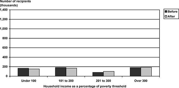
SSI recipients whose benefits are increased under option 7/0: Poverty distribution before and after simulation
| Household income as a percentage of poverty threshold |
Number of recipients | |
|---|---|---|
| Before | After | |
| Under 100 | 167,881 | 153,027 |
| 101 to 200 | 182,533 | 169,512 |
| 201 to 300 | 80,766 | 101,945 |
| Over 300 | 181,099 | 187,793 |
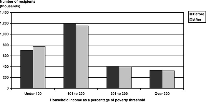
SSI recipients whose benefits are reduced under option 7/0: Poverty distribution before and after simulation
| Household income as a percentage of poverty threshold |
Number of recipients | |
|---|---|---|
| Before | After | |
| Under 100 | 703,970 | 772,700 |
| 101 to 200 | 1,201,914 | 1,155,041 |
| 201 to 300 | 411,447 | 398,944 |
| Over 300 | 334,761 | 325,414 |
Under 7/0, recipients with reduced benefits outnumber those with increased benefits, 41 percent to 9 percent (Chart 5). This difference in the size of the groups, combined with how the groups are distributed above and below the poverty threshold, accounts for the poverty outcomes that we observe. As shown above, those with benefit increases under 7/0 have high incomes relative to other SSI recipients—over 70 percent have incomes above the poverty threshold (see Table 3 and Charts 7 and 8). By implication, because of their small numbers and because the majority of them have incomes above the poverty threshold (see Chart 7), their benefit increases have limited impact on the poverty rate. The poverty outcomes, then, mainly reflect the income changes of those with benefit reductions. Over 40 percent of recipients with benefit reductions have incomes just above the poverty threshold, in the 101 percent to 200 percent bracket (see Chart 8). Chart 8 shows that those with benefit reductions appear along a broad segment of the income distribution scale. There is a general shift downward, and enough of those just above the threshold fall into poverty—moving from just above the threshold to just below—to account for the overall poverty rate increase of 1.5 percentage points (see Chart 9 and Table 4). Hence, because those with benefit increases have higher household incomes than those with reductions, benefit restructuring, although well-suited to simplifying ISM, is poorly designed for reducing poverty.19
Combining SSI recipients whose benefits are increased and reduced under option 7/0: Poverty distribution before and after simulation
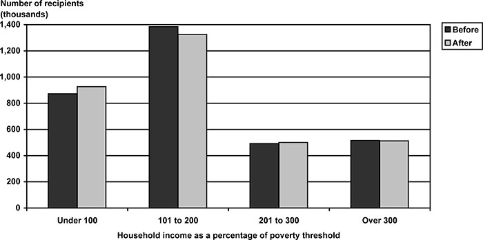
| Household income as a percentage of poverty threshold |
Number of recipients | |
|---|---|---|
| Before | After | |
| Under 100 | 871,854 | 925,724 |
| 101 to 200 | 1,384,447 | 1,324,553 |
| 201 to 300 | 492,212 | 500,888 |
| Over 300 | 515,860 | 513,207 |
The poverty outcomes for 10/5 are counterintuitive: Why would poverty rates increase by 2.2 percentage points if benefits are increased both for recipients receiving ISM (Chart 10) as well as for recipients living alone, a subgroup with a 90 percent poverty rate (see Chart 11 and Table 4)? There are two reasons. First, under 10/5 those in shared housing have a 10 percent reduction in the SSI income guarantee, resulting in a 2.9 percentage-point increase in poverty for a group that includes almost half of all SSI recipients (see Table 4 and Chart 12). Second, although those living without other adults have a 2.5 percentage-point reduction in poverty, more detailed estimates show that many in this group have incomes well below the poverty threshold; hence, while a 5 percent increase in the FBR makes them better off, it does not bring many of them out of poverty. We confirmed this from unpublished tabulations showing a 12 percent reduction for those with incomes at or below 75 percent of the poverty threshold. Although the effect on the poverty rate is modest, the poverty gap measure registers the improvement. Under 10/5 the poverty gap is reduced by 2.7 percent, and for those living alone it is reduced by 18 percent (see Table 4). The 10/5 proposal links benefit increases related to benefit restructuring to separate increases for those living alone, but unpublished tabulations show stark differences between the two types of benefit increases with respect to their effectiveness in reducing poverty. Specifically, 87 percent of those with benefit increases related to ISM elimination are nonpoor (see Chart 10). Conversely, under the 5 percent FBR increase for those living alone, 87 percent of those with benefit increases are poor (compare Charts 10 and 11). Chart 13 shows the net effect of 10/5.
SSI recipients whose benefits are increased (charged with ISM) under option 10/5: Poverty distribution before and after simulation
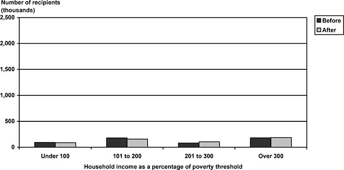
| Household income as a percentage of poverty threshold |
Number of recipients | |
|---|---|---|
| Before | After | |
| Under 100 | 92,327 | 86,202 |
| 101 to 200 | 178,293 | 156,545 |
| 201 to 300 | 80,765 | 104,187 |
| Over 300 | 181,103 | 185,553 |
SSI recipients whose benefits are increased (living alone) under option 10/5: Poverty distribution before and after simulation
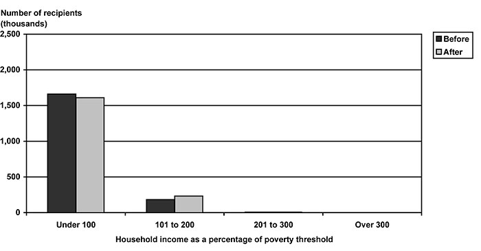
| Household income as a percentage of poverty threshold |
Number of recipients | |
|---|---|---|
| Before | After | |
| Under 100 | 1,660,718 | 1,610,207 |
| 101 to 200 | 182,125 | 232,604 |
| 201 to 300 | 7,136 | 7,136 |
| Over 300 | 0 | 0 |
SSI recipients whose benefits are reduced under option 10/5: Poverty distribution before and after simulation
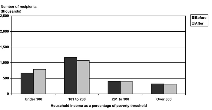
| Household income as a percentage of poverty threshold |
Number of recipients | |
|---|---|---|
| Before | After | |
| Under 100 | 666,598 | 787,282 |
| 101 to 200 | 1,166,715 | 1,069,461 |
| 201 to 300 | 404,503 | 390,179 |
| Over 300 | 320,434 | 311,329 |
Combining SSI recipients whose benefits are increased and reduced under option 10/5: Poverty distribution before and after simulation
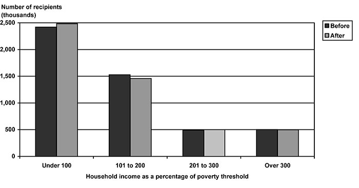
| Household income as a percentage of poverty threshold |
Number of recipients | |
|---|---|---|
| Before | After | |
| Under 100 | 2,419,643 | 2,483,691 |
| 101 to 200 | 1,527,132 | 1,458,610 |
| 201 to 300 | 492,404 | 501,502 |
| Over 300 | 501,537 | 496,882 |
The poverty effects vary by subgroup, especially for living arrangement groups (see Table 4).20 As mentioned above, under 7/0 adult recipients living with adults other than eligible spouses (49 percent of all recipients) would have an increase in the poverty rate of 1.5 percentage points and an increase in their poverty gap of 7.3 percent. Under 10/5, the poverty gap would be reduced by 18 percent for adults living without other adults in their households—the group benefiting from a 5 percent increase in the FBR. But the largest group—adult recipients living with other adults and subject to the 10 percent reduction—would experience an increase in poverty. The poverty rate for this group would increase by 2.9 percentage points and the poverty gap would increase by 13.9 percent. Under 10/5, elderly and female recipients would have marked reductions in the poverty gap because they are overrepresented among those with FBR increases (those living without other adults) and underrepresented among those with reductions (especially those living with other adults).
Conclusion
The ISM and living arrangement policies now in place are highly complex, requiring program administrators to establish living arrangement categories for all recipients and receipt of ISM for most recipients. This implies detailed tracking of household expenses, the recipient's contribution to household expenses, and how the recipient's contribution is earmarked within the household budget. By contrast, under benefit restructuring, program administrators would avoid the minutiae of household budgeting altogether—by simply establishing whether the recipient lives with another adult. If so, administrators would compute benefits using a reduced FBR; otherwise, they would use the full FBR.
Current policy and the alternative analyzed here—benefit restructuring—have distinct rationales. Under current policy, benefits are reduced to partially offset the receipt of ISM for about 9 percent of recipients, reflecting a fundamental program equity goal. By contrast, under benefit restructuring there would be no benefit reductions for those receiving in-kind support from family or friends. However, to recoup the higher benefits paid to those now receiving ISM, recipients who share housing—roughly half of all recipients—would be assessed benefit reductions. These reductions would target adults who share housing, on grounds that they are better off than most recipients because of economies of scale in housing, utilities, and food.
For both current policy and benefit restructuring, incentive effects follow from how the benefit reductions are targeted. Current policy probably discourages in-kind contributions, especially for those who might make smaller contributions because such contributions trigger a dollar-for-dollar benefit reduction. Benefit restructuring would undo such disincentives, encouraging in-kind contributions. In addition, current policy may provide a disincentive to share housing for SSI recipients faced with the one-third reduction. Analogously, benefit restructuring may create a disincentive to share housing for those subject to a reduced FBR.
The effects of eliminating ISM-related benefit reductions can be disentangled from the effects of recouping revenues from those who share housing. Eliminating ISM, taken alone, would simplify program administration (saving about $70 million per year), encourage contributions to recipients, and substantially increase benefits for recipients currently receiving contributions of food or shelter—but at a cost of roughly $1.2 billion annually. Because of budget neutrality, those costs must be recouped and, under benefit restructuring, they are recouped through benefit reductions to recipients who share housing. One concern is that this large-scale redistribution—affecting $1.2 billion of annual benefits and 50 percent to 75 percent of all recipients—may be considered disproportionate to the $70 million annual cost of administering ISM.
Yet another concern is the broad redistributional and poverty outcomes of benefit restructuring. Under 7/0—benefit restructuring in its purest form—the 9 percent of recipients with ISM would have benefit increases averaging 44 percent, or $164 per month. The associated program costs would be offset by a 9 percent average benefit reduction ($44 per month) for 41 percent of all recipients—those who share housing. And, because a higher percentage of the disabled share housing than do the aged, disabled adults would bear a somewhat disproportionate share of the benefit reductions. Furthermore, although both those with benefit increases and benefit reductions have lower poverty rates than the average SSI recipient, we find that—even before any changes in benefits—the household incomes of those with benefit increases would be 42 percent higher than the household incomes of recipients with benefit reductions. In addition, there are increases in poverty under both the 7/0 option (1.5 percentage points) and the 10/5 option (2.2 percentage points), and under 7/0, the great majority of those with benefit increases would be nonpoor. Hence, the broad distributional outcomes for benefit restructuring are not consistent with the underlying distributional objective of SSI—to provide more assistance to those most in need.
A special provision under 10/5 does reduce poverty for a key subgroup, closing the poverty gap for individuals living alone or with minor children. This group comprises 27 percent of all SSI recipients, disproportionately women and the elderly, and it has an initial poverty rate of 90 percent. Although this provision does not contribute to ISM simplification, it reduces poverty quite efficiently. But, one might ask whether it is equitable that recipients in shared housing should bear its cost.
How can we simplify current ISM and living arrangement policies, but avoid the redistributional and poverty outcomes reported here? Accepting budget neutrality as a given probably implies dropping total elimination of ISM as a policy option. Instead, future research might consider incremental reforms of current ISM policy that do not entail large-scale redistribution of benefits.
Appendix: Simulation Methodology
The simulation results are derived from the Financial Eligibility Model (FEM)—a static simulation model developed by the Office of Policy (currently the Office of Retirement and Disability Policy) staff and used in several previous studies (see Wixon and Vaughan (1991); Davies and others (2001/2002); Rupp, Strand, and Davies (2003); and Davies, Rupp, and Strand (2004)). The FEM has undergone substantial enhancement in order to address the subject of this Supplemental Security Income (SSI) benefit restructuring study. The Social Security Administration (SSA) beneficiary data from the Revised Management Information Counts System (REMICS) have been added to the FEM. Linking these administrative records with survey data allows researchers to identify those receiving in-kind support and maintenance (ISM) and the amounts received. Potential ISM status is then imputed via a hot deck process to a portion of the nonparticipants who could be eligible for SSI under any of the reform scenarios.
A static simulation model is designed to assess changes in the size and characteristics of the recipient population that might reasonably be anticipated to occur as a result of specific changes in program parameters. The model allows people to enter the rolls if they become newly eligible or if their potential benefit amounts increase. Similarly, people leave the rolls if they lose eligibility, and they may leave if their benefits decrease. The simulations assume that only changes in specific program parameters affect outcomes and that all of the changes occur instantaneously. In other words, the model holds constant SSA policies (other than the policy parameters altered by any given policy scenario) and the characteristics of the target population, and it reflects full implementation of and complete adjustment to the reform scenario by SSA staff and by potential and actual recipients. The model assumes that the behavior of the target population and the way in which SSA staff administer the program do not change except in response to changes in program eligibility and benefit levels. These are restrictive assumptions, but also very useful ones in that they help focus on the likely implications of the proposed reforms rather than other changes over time in recipient characteristics and behavior, as well as program operations.
The FEM is based on the Survey of Income and Program Participation (SIPP) exact matched to SSA administrative records using Social Security numbers reported by survey respondents. The survey estimates reflect the noninstitutional population of the United States, and all data represent the reference month of November 1996. The Supplemental Security Record data are the source of information on current-pay status and monthly federal benefits for participants. Whether ISM is received and the degree to which benefits are reduced for ISM are taken from the REMICS. All of the estimates are weighted to reflect the underlying study universe of people. The FEM produces percentage differences in SSI enrollment between a given proposal and the status quo. These percentages are then applied to actual or projected SSI enrollments to generate changes in SSI rolls associated with the proposal. In this study, estimated percentage changes in SSI enrollment were applied to the December 2005 SSI population for the age categories represented here: 0 to 17, 18 to 64, and 65 or older. This allows the policymaker to obtain a reasonably accurate sense of the changes that would have occurred in December 2005 as a result of full implementation of a proposed policy change.
A key component of the FEM is the SSI benefit calculator. Calculated benefits are based on SIPP-reported earned and unearned income and other characteristics related to the SSI eligibility determination. The benefit calculator uses program parameters and rules to calculate an expected federal SSI benefit amount. Those sample members with positive calculated federal benefits are deemed payment eligible. If payment-eligible individuals participate in SSI, they are presumed to receive any state supplements that would be available to them as well as the federal benefits calculated from the SIPP source data. The calculated payment, eligibility status, and potential (or expected) monthly federal benefit are available for all members of the relevant SIPP sample, whether the sample member actually participated in the program or not. This is important because not all SSI eligibles choose to enroll in the program, and also because payment eligibility and expected federal payment amounts may change as a result of simulated changes. For each simulation, the benefit calculator estimates eligibility and federal benefits under two scenarios: (1) the "baseline scenario," reflecting status quo program rules, and (2) a "simulation scenario," reflecting hypothetical changes in program rules. For example, a simulation scenario may eliminate ISM and increase or decrease the federal benefit rate (FBR) for specific classes of potential recipients by a predetermined percent value. Finally, the relevant differences between the baseline scenario and the simulation scenario are calculated, and all simulation outcomes of interest (such as household income and poverty status) are recalculated to reflect simulated changes in participation status and monthly federal benefits.
Because not all eligibles participate under current conditions, it is reasonable to assume that the same is true for the simulation scenario. Participation status may change as a result of changes in eligibility status, financial incentives, and possibly other factors such as stigma. The model predicts participation separately for elderly and disabled adults using a multivariate model (probit equation) that posits that participation is a function of various recipient characteristics, environmental factors, and financial incentives arising from the dollar value of expected benefits. It is assumed that, other things equal, participation is more likely if expected federal SSI benefits are relatively high. The parameters from the model that was estimated using baseline conditions are then applied to the pool of eligibles and the value of the independent variables under the simulation scenario. By construction, all variables other than expected SSI benefits (and by implication, payment eligibility status) are presumed to equal baseline conditions. Importantly, the model does not presume that the rate of participation is unchanged between the baseline and simulation scenarios, but allows the probability and overall rate of participation to vary in response to changes in expected benefits between the two scenarios. Note that expected benefits for some adults may increase (as a result of the elimination of ISM and increased FBR for some), although they may decrease for others (as a result of a simulated FBR reduction not sufficiently counterbalanced by the elimination of ISM, to maintain or increase baseline benefits). The simulations reflect the net result of ISM and FBR changes.
In order to receive SSI, individuals must meet categorical eligibility requirements by either being blind, disabled, or older than age 65. Although it would be difficult to determine precisely which unenrolled individuals meet SSA disability standards, this sort of determination is generally not necessary for a participation model. Rather, participation is estimated directly as a function of financial and disability-related characteristics. It turns out that the eligible spouse category is dominated by elderly couples, whose categorical eligibility is not in question. However, the identification of adult recipients living with ineligible spouses younger than age 65 is questionable and can be estimated only with substantial measurement error. Adults with ineligible spouses also form the smallest of the living arrangement categories identified in this analysis. For these two reasons combined, no detailed results are presented for this subgroup.
Calculations for deeming the income of an ineligible spouse would change as a result of changes to the benefit rate under benefit restructuring. An SSI applicant or recipient with an ineligible spouse must qualify on the basis of his or her own income before any deeming of the spouse's income is considered. If the ineligible spouse's income is less than the difference between the individual and couple FBR, there is no income to deem and the eligible individual's own income is subtracted from the individual FBR to determine the benefit amount (calculation 1). If the ineligible spouse's income is greater than the difference between the two benefit rates, the eligible individual and ineligible spouse are treated as an eligible couple for purposes of counting income (calculation 2). Before incomes are combined, an allocation for each ineligible child equal to the difference between the FBR for a couple and the FBR for an individual is subtracted from the ineligible spouse's income. The basis for this allocation would not change under benefit restructuring. All of the options would use the reduced FBR for an individual living with another adult in the first calculation.
Modeling participation among eligible children is a technically difficult objective that has not been achieved to date. Instead, we begin with the observed pool of child recipients and assume that changes to this group will be similar to those estimated for adults. For each simulation scenario, we calculate the factor by which the recipient population changes for unmarried adults living with other adults, and we apply this same factor to the recipient population for children. Because the proposed reforms do not change the FBR for children, results presented in this study are not substantially affected by this assumption. Nevertheless, a limitation of our approach is that we do not estimate the characteristics of children who would become newly eligible as a result of the elimination of ISM.
In the current simulation exercise, FBR reductions were chosen to avoid increasing simulated SSI program costs under full implementation. For example, the 7/0 option is presented because 7 is the smallest whole percentage-point FBR reduction for adults that covers the cost to SSI of eliminating ISM-related benefit reductions, according to the FEM. Because only whole percentage-point FBR reductions are considered, we would actually expect some very minor long-term SSI savings for the proposed reforms. The FEM does not consider administrative costs or savings, nor does it capture costs or savings to other programs such as Medicaid.
Notes
1 In this analysis we use "income guarantee" and "FBR" interchangeably.
2 As of 2004, 47 states and the District of Columbia supplement the federal SSI payment. The amount of state supplementation varies by the living arrangement of the recipient and by state. In fact, six states (California, Massachusetts, New York, North Carolina, Pennsylvania, and Wisconsin) account for 84 percent of all supplement dollars paid.
3 Because the SSI benefit is included in household income when calculating the amount of food stamps for a household, an increase or decrease in the SSI payment would generate a countervailing effect on the Food Stamp Program (FSP) grant for those receiving food stamps. FSP changes would offset about 30 percent of the change in SSI benefits.
4 This article uses a household poverty measure, rather than the conventional family based poverty measure. The family based measure may be biased in the following respect. In some cases an SSI recipient may reside with an unrelated person, enjoying economies of scale with respect to costs of shelter and utilities. Current policies for counting ISM do not distinguish between households of unrelated persons and family households. Using a family based measure implies that the poverty threshold used in calculating poverty for the SSI recipient or couple will not reflect such economies of scale (because the recipient and roommate are unrelated) and the resulting poverty estimates may be too high. By contrast, using a household-based measure would capture the effects of such economies, resulting in lower poverty rates. In fact, for the largest household composition category used in this analysis—adults living with other adults—using a household measure of poverty reduced poverty rates in our sample from 38 percent to 24 percent. However, there is also good reason to believe that a household-based measure yields poverty estimates that are too low. The household-based measure assumes that the income of all household members is equally available to meet the needs of all household members, that is, there is full sharing of income. In this respect, the household measure is not consistent with the conventional family measure that assumes family members share income, but unrelated persons do not. Also, using the household-based measure makes it problematic to compare poverty estimates from this analysis with conventional poverty estimates.
5 Report of the Committee on Finance, United States Senate, to accompany H.R. 1, September 26, 1972.
6 If the recipient has no other income, the first $20 of ISM received under the PMV may be excluded using the general income exclusion. The examples that follow assume that the recipient has other unearned income, so the $20 exclusion would not be available to offset any ISM received.
7 The $20 general income exclusion may be applied to earnings (raising the initial exclusion to $85) provided the recipient does not have unearned income to which the exclusion would be applied.
8 Cost estimates are for 2007, based on unpublished estimates by SSA's Office of the Chief Actuary, dated October 31, 2005.
9 Final regulations were published on February 7, 2005.
10 The benefit reductions would not extend to eligible couples, on grounds that the benefit for such couples currently reflects economies of scale from shared housing. Eligible couples receive benefits based on 150 percent of the individual-guarantee level, rather than 200 percent.
11 Costs could increase if an implementation strategy is used, for example, to protect the benefits of current recipients. No implementation strategies are simulated in this analysis, nor are Medicaid cost increases factored into the cost estimates.
12 A simpler process is used for institutionalized applicants.
13 Office of Budget estimate, May 4, 2006.
14 SSI recipients can receive large ISM contributions under current policy. That would not change under the options analyzed here. For example, policymakers should be aware that under both current policies and the options being considered, parents could maintain an adult child receiving SSI in a high rent apartment, paying the rent, food, and utilities. That said, the new options would clearly encourage additional contributions of food or shelter, especially contributions of modest amounts.
15 Chart 6 shows that 7 percent of recipients have ISM, rather than the 9 percent shown in Chart 5. This difference mainly reflects a number of recipients who live alone and receive ISM. In chart 1, those individuals are included in the ISM group, and in chart 6 they are classified as living alone.
16 In some cases, those exiting or entering the program may have low SSI benefits, but their Medicaid benefits make them a key subgroup in terms of budgetary effects. This analysis does not take into account Medicaid costs.
17 We classify affected groups by the net effect of the policy options—whether the recipient's total benefit is increased or reduced.
18 Furthermore, for disabled adults with benefit increases, the initial household income is over 50 percent greater than for those with benefit decreases (from unpublished tabulations).
19 Note that recipients in extreme poverty—with incomes less than 50 percent of the poverty threshold—increase by over 50 percent under both options. Many of these recipients appear to be living with other adults who have little or no income and, under benefit restructuring, their benefits would be reduced. Although such recipients comprise only a fraction of those affected by benefit restructuring (3 percent under option 7/0), they gain nothing from the economies of scale from sharing housing because their roommates are indigent.
20 Stark differences for living arrangement groups are not surprising. Under both proposals, benefit increases and reductions are targeted explicitly by living arrangement.
References
Davies, Paul S., Minh Huynh, Chad Newcomb, Paul O'Leary, Kalman Rupp, and Jim Sears. 2001/2002. Modeling SSI financial eligibility and simulating the effect of policy options. Social Security Bulletin 64(2): 16–45.
Davies, Paul S., Kalman Rupp, and Alexander Strand. 2004. The potential of the Supplemental Security Income program to reduce poverty among the elderly. Journal of Aging and Social Policy 16(1): 21–42.
[GAO] Government Accountability Office. 2002. Supplemental Security Income: Progress made in detecting and recovering overpayments, but management attention should continue. Report No. GAO-02-849 (September).
Rupp, Kalman, Alexander Strand, and Paul Davies. 2003. Poverty among elderly women: Assessing SSI options to strengthen Social Security reform. Journal of Gerontology: Social Sciences 58B(6): S359–S368.
[SSA] Social Security Administration. 2000. Simplifying the Supplemental Security Income program: Challenges and opportunities. SSA Pub. No. 13-005. Office of Policy.
————. 2005. Annual report of the Supplemental Security Income program. Social Security Advisory Board statement on the Supplemental Security Income program. Office of the Chief Actuary (October).
————. 2007a. Payment accuracy (stewardship) report: Supplemental Security Income, fiscal year 2006. Office of Quality Performance (September).
————. 2007b. SSI annual statistical report, 2006. Office of Policy. Office of Research, Evaluation and Statistics.
————. 2008. Characteristics of noninstitutionalized DI and SSI program participants. Research and Statistics Note No. 2008-02. Office of Policy, Office of Research, Evaluation, and Statistics (January).
Wixon, Bernard, and Denton Vaughan. 1991. Rationale for a SIPP-based microsimulation model of SSI and OASDI. ORS Working Paper Series No. 54. Washington, DC: Social Security Administration.