The Longevity Visualizer: An Analytic Tool for Exploring the Cohort Mortality Data Produced by the Office of the Chief Actuary
Research and Statistics Note No. 2016-02 (released May 2016)
The author is with the Office of Policy Analysis, Office of Retirement Policy, Office of Retirement and Disability Policy, Social Security Administration.
Acknowledgments: I thank Michael Morris, Mark Bye, Tiffany Bosley, Steve Goss, Teresa Daniels, Dale Kintzel, Patrick Purcell, and Mark Sarney for their helpful comments and suggestions for both the manuscript and the LV software.
The findings and conclusions presented in this note are those of the author and do not necessarily represent the views of the Social Security Administration.
Introduction
| LV | Longevity Visualizer |
| OASDI | Old-Age, Survivors, and Disability Insurance |
| OCACT | Office of the Chief Actuary |
In the Annual Report of the Board of Trustees of the Federal Old-Age and Survivors Insurance and Federal Disability Insurance Trust Funds (hereafter, the Trustees Report), the Social Security Administration's Office of the Chief Actuary (OCACT) estimates the future finances of the Old-Age, Survivors, and Disability Insurance (OASDI, or Social Security) program and other federally administered insurance programs. Mortality-rate projections for the Social Security coverage population are critical for assessing the future health of the program. OCACT produces various mortality-rate formulations, one of which is a data set known as the cohort life tables. Those tables project the fraction of the population born in a given calendar year that will remain alive at each annual age in the future. In so doing, they also indicate the probability that a member of that birth cohort will die at each annual age.
Although OCACT produces them to project Social Security system finances, the life tables can also inform individual decisions that rely on an understanding of potential longevity. Publicly available life-expectancy calculators typically provide only summary measures, such as the average number of years of life remaining at given ages—and perhaps the median and quartile values for years remaining—but they generally do not provide the full age-at-death probability distributions. Most calculators also cannot support the joint-probability queries that provide dual longevity projections, such as those for a married couple planning their retirements. Cohort life tables can provide all of that information; however, individual users might find the tables difficult to understand and cumbersome to navigate. To make this rich data set and its analytical potential more accessible to the interested public, the Social Security Administration has incorporated the cohort life-table data into an interactive software package called the Longevity Visualizer (LV). This note introduces the LV, describes its computational methodology and the analyses it can perform, and provides examples of its data visualization capabilities.
Cohort Life Tables
The LV uses the cohort life tables prepared by OCACT for the intermediate-case projections of the 2015 Trustees Report.1 These tables include, for each birth year from 1850 through 2075 and for males and females separately, both the historical and projected mortality rates at each annual age from 0 to 120. In the context of the LV, a cohort is the population of a given birth year and sex (for example, the cohort of all females born in 1922). A record in this data set is indexed by birth year, sex, and current age.2 Each record includes a number of variables related to mortality; however, the LV uses only (the probability that an individual aged years will die within 1 year) and (the expected number of years of life remaining for an individual aged years). All LV computations, including survival functions, age-at-death probability distributions, and expected age at death, are derived from those two variables. Appendix A documents the full specification of the LV computations. Bell and Miller (2005) provide general documentation of the original life tables, with definitions of the variables and a description of the calculations used in their computation.
Overview of the Software
The LV is a Microsoft Windows application developed with Microsoft C# 5.0 and .NET Framework 4.5. All data necessary for the computations are embedded in the application's executable file so that no database or external storage is required for deployment. The user interface is organized into six tabs:
- Survival;
- Probability of Death;
- Multi-Cohort Survival;
- Gender Gap;
- Joint Survivability; and
- Basic Functions.
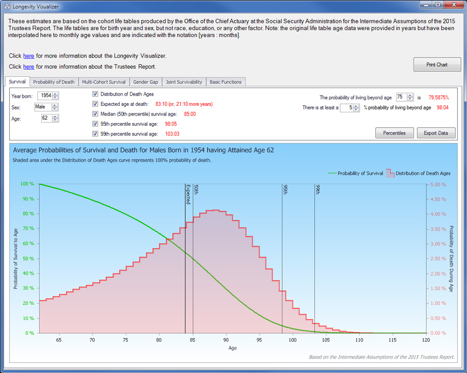
The sections below discuss the functions of the tabs, with sample screen shots and examples of the charts the LV can produce. The illustrations generally assume a hypothetical male subject born in 1954, who is thus aged 62 (the earliest age for claiming OASDI retirement benefits) in 2016.
Cohort Survival Functions
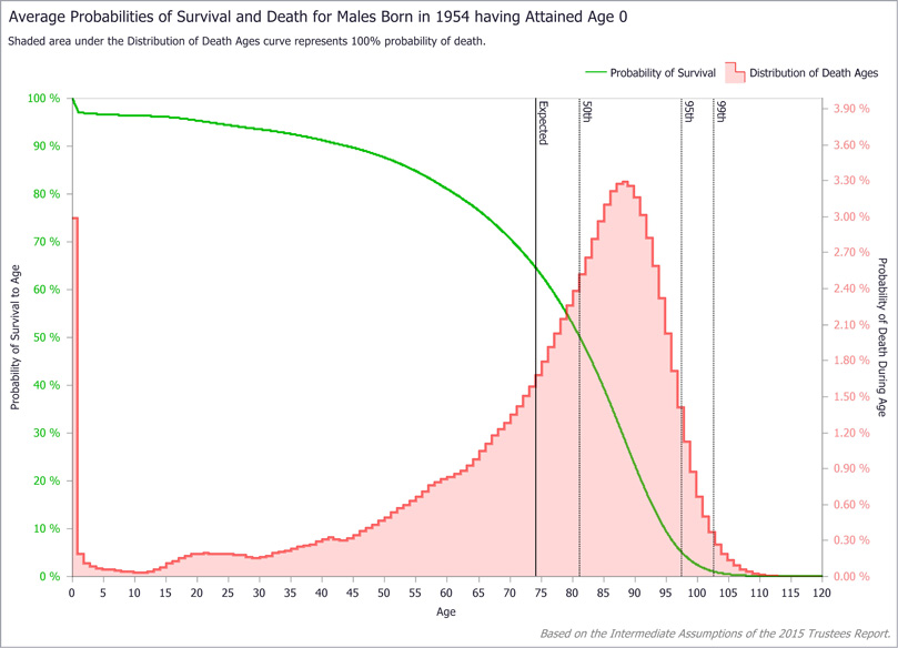
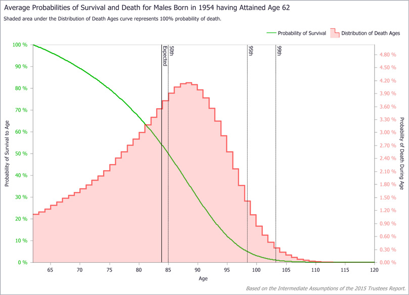
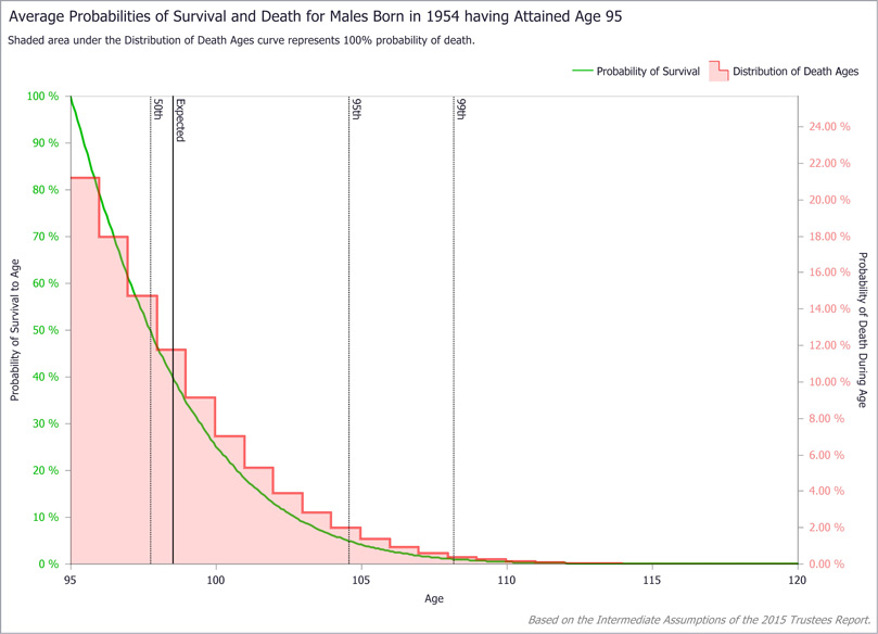
The Survival tab (Exhibit 1) produces a composite survival chart along with selected statistics for an individual of a given cohort and current age. Exhibits 2–4 show composite charts for the subject (male born in 1954) at birth, age 62, and age 95, respectively. The survival probability function in each chart starts with 100 percent survivability at the current age and decreases monotonically to 0 percent survivability at age 120. Note that survivability decreases more rapidly with advancing current age, particularly by age 95.
Underlying the survival curve in each composite chart is the age-at-death probability distribution. The most striking feature of the plots is the strong asymmetry of the distributions. Although the distributions are generally bell-shaped at birth (Exhibit 2) and at age 62 (Exhibit 3), negative skew tilts toward death at younger ages. Distributions for all current ages are asymmetric, but the general bell shape disappears at advanced ages, as can be seen at age 95 (Exhibit 4), when the sample subject is more likely to die at his current age than at any other.
LV Survival tab: Illustrative screen shot
LV Survival tab: Sample query results (composite survival chart for a male subject born in 1954 at age 0)
LV Survival tab: Sample query results (composite survival chart for a male subject born in 1954 at age 62)
LV Survival tab: Sample query results (composite survival chart for a male subject born in 1954 at age 95)
The Probability of Death tab (Exhibit 5) further explores changes in the age-at-death probability distribution for a given individual over his or her lifetime. Those changes may have implications for retirement decision making. For instance, suppose the sample subject (male born in 1954, currently aged 62) is deciding at which age, from 62 through 70, to claim retirement benefits. Because his cohort's life expectancy age is about 84 years, he may target 84 as the lifetime-benefit breakeven age (described later) that underlies his claiming decision. The gray box in the lower left corner of Exhibit 5 shows that at age 62, the probability that he will survive to age 84, designated as D>83, is 53.70 percent; should he reach age 70, however, the probability at that point that he will survive to age 84 is 60.26 percent. That progression is intuitive: For each successive year that an individual survives, the probability of reaching a fixed target age increases. Inversely, at age 62, the subject has a 46.30 percent chance of dying before reaching age 84 (D≦83) and a 10.89 percent chance of dying before age 70 (D<70); the difference (35.41 percent) thus represents his probability, at age 62, of dying aged 70–83 (70≦D≦83). However, if he survives to age 70, then at that point his probability of dying aged 70–83 is 39.74 percent—substantially higher than it was at age 62.
LV Probability of Death tab: Illustrative screen shot
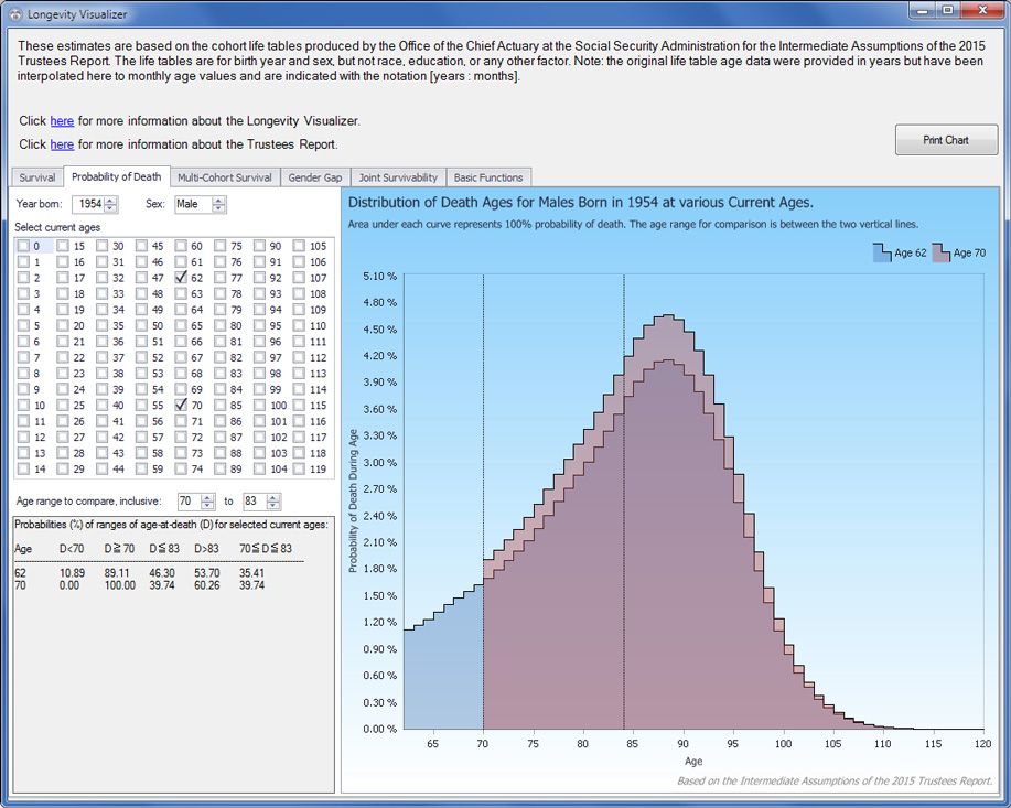
How can the probabilities of death before age 84 and survival to age 84 both increase as one ages from 62 to 70? The explanation begins with the obvious tautology of a 100 percent chance of dying sometime between one's current age and a given maximum possible death age (120 in the LV) to which no one, statistically speaking, survives. Thus, for a current 62-year-old, the total probability of death between ages 62 and 120 is 100 percent, as is the total probability of death for a current 70-year-old between ages 70 and 120. Because surviving to age 70 precludes the probability of dying aged 62–69, that 10.89 percent probability transfers to a now-compressed range of possible death ages. Even though the probability of living to age 84 has increased for the 70-year-old, the former probability of death at ages 62–69, now transferred forward, inflates the probability of death at ages 70–83 (and all ages through 120), as illustrated by the chart in Exhibit 5. This circumstance complicates the retirement decision: As one ages, the critical age-specific probabilities of death and survival increase in tandem.
A notable application of the survival functions is the calculation of lifetime Social Security retirement benefits for the range of permissible claiming ages from 62 through 70. Claiming benefits at younger ages of eligibility reduces the monthly benefit amount, but extends the number of years over which benefits are collected. Conversely, delayed claiming increases the monthly benefit but reduces the number of years of collection. Broadly speaking, a beneficiary who dies before his expected age of death is better off having claimed benefits earlier; one who survives longer is better off having delayed claiming. If one dies at exactly the age of life expectancy, then the lifetime present value of benefits is roughly the same regardless of claiming age (Meyer and Reichenstein 2010). Nevertheless, the redistribution of death-age probabilities as one ages poses a considerable risk. For instance, if the sample subject decides to delay claiming from age 62 until age 70, he must not only survive another 8 years to reach his planned claiming age; he must also overcome the probability of dying during the critical recouping ages of 70 through 84, which is then elevated precisely because he was fortunate enough to survive to age 70 in the first place. In other words, the 70-year-old claimant must survive another 14 years—during which he faces an increasing age-specific probability of death—before his lifetime benefits equal what they would have been if he had claimed at age 62. Deciding when to claim is not straightforward, even for the singular consideration of maximizing one's expected lifetime benefits.3
Multi-Cohort Survival, Gender Gap, and Basic Function Analyses
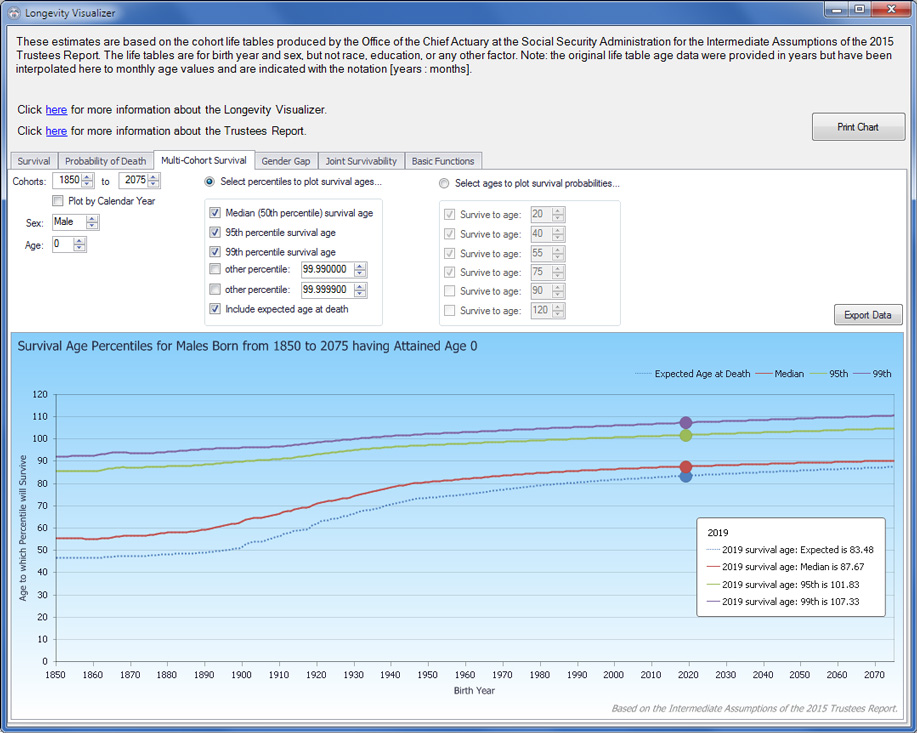
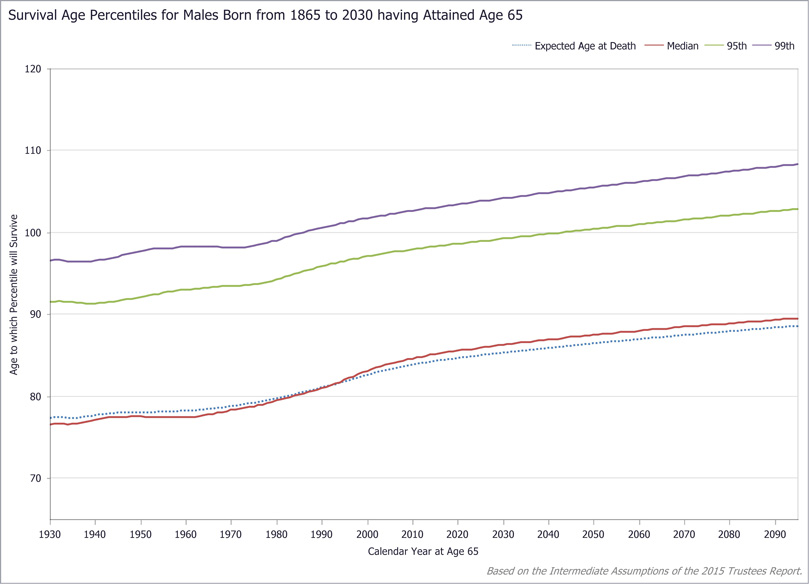
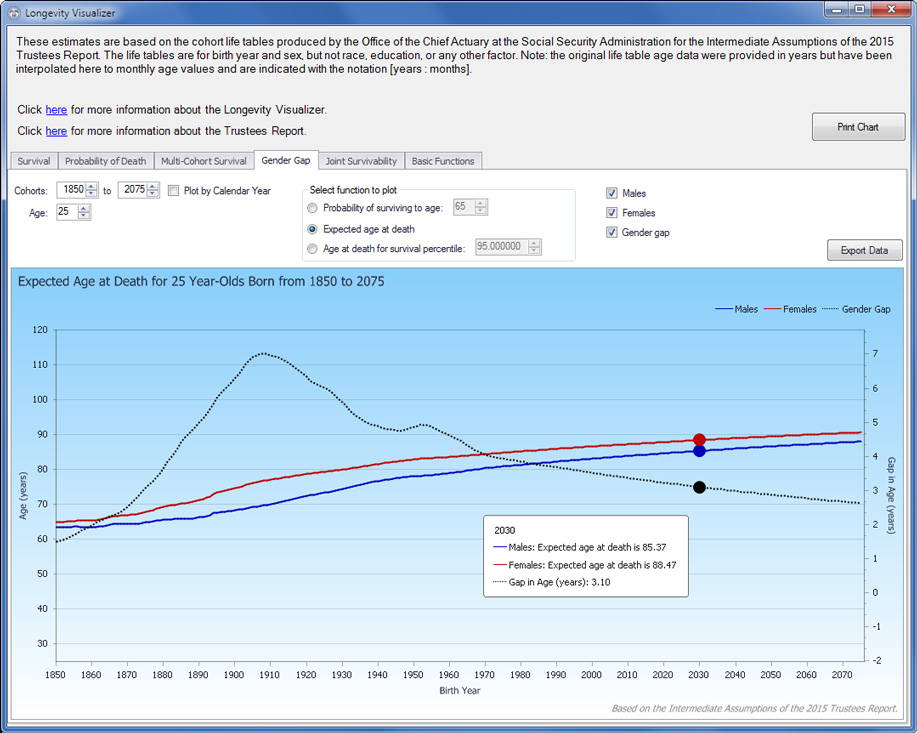
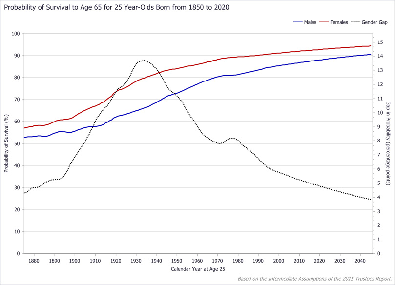
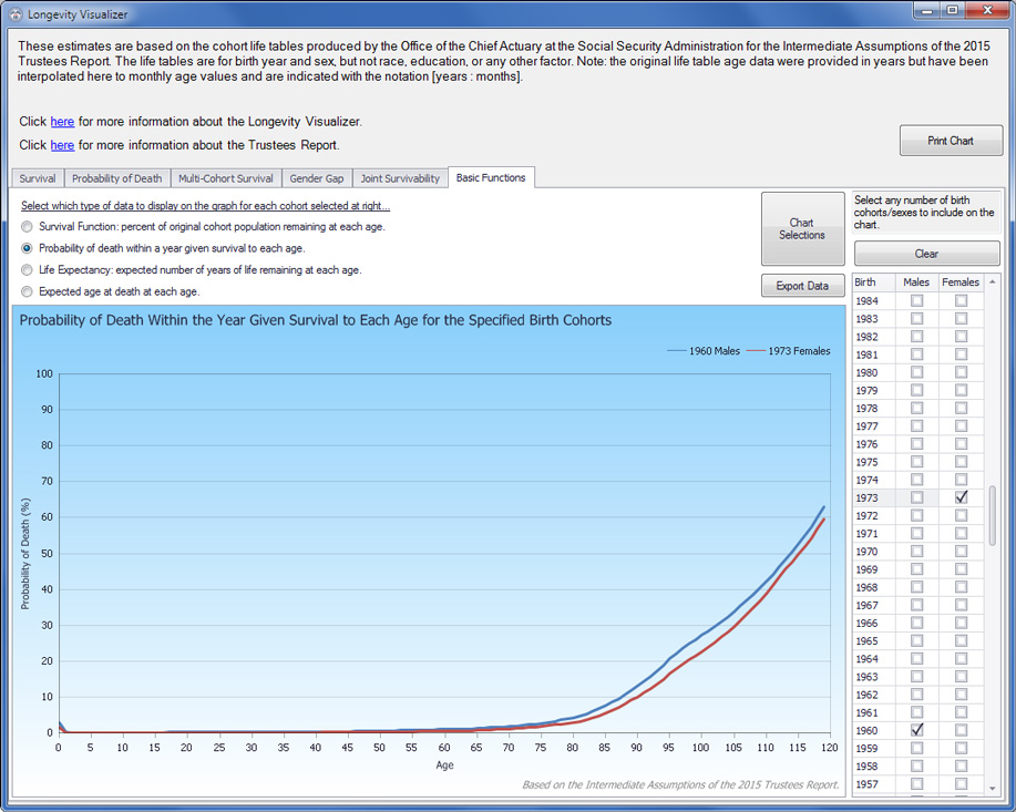
These three tabs demonstrate the LV's capability for multi-cohort longevity analyses. In the Multi-Cohort Survival tab (Exhibit 6), users can compare numerous measures of survival across multiple birth-year cohorts for subjects of the same sex and current age. Exhibit 7 shows the plot of various percentiles (and the mean, or expected value) of survival age for current 65-year-old males born from 1865 through 2030. Clearly, improvements in life expectancy, notably for individuals at older ages, increase survival projections over successive cohorts. Without attempting to interpret the percentile fluctuations over the twentieth century, one can see a steady rise of all percentiles beginning in the 1970s. The Gender Gap tab (Exhibit 8) enables comparisons across multiple birth-year cohorts of specific survival-age probabilities, the expected age at death, and specific survival percentiles for both men and women as well as the gap between them. Exhibit 9 shows the probability of a 25-year-old of each sex surviving to age 65 across birth cohorts from 1850 through 2020, indicating the likelihood of surviving to retirement age for individuals still in their early years of labor force participation. The Basic Functions tab (Exhibit 10) offers a set of related capabilities, with which any number of cohorts can be compared by survivability, probability of death, and life expectancy, at all current ages from birth to 120.
LV Multi-Cohort Survival tab: Illustrative screen shot
LV Multi-Cohort Survival tab: Sample query results (survival probabilities for males aged 65, 1865–2030 cohorts)
LV Gender Gap tab: Illustrative screen shot
LV Gender Gap tab: Sample query results (probability of surviving to age 65, current 25-year-olds born 1850–2020, by sex)
LV Basic Functions tab: Illustrative screen shot
Joint Survivability
The Joint Survivability tab (Exhibit 11) enables analysis of joint survival probabilities of two persons.4 These joint probabilities comprise all possible future combinations of life and death for the two persons given the cohort for each and a calendar year (and thus the current age of each). The joint probabilities are calculated directly from the survival function of each person at his or her current age. Appendix B presents the formulae for all possible joint probabilities.
LV Joint Survivability tab: Illustrative screen shot
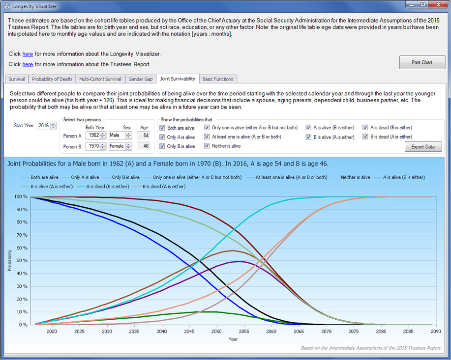
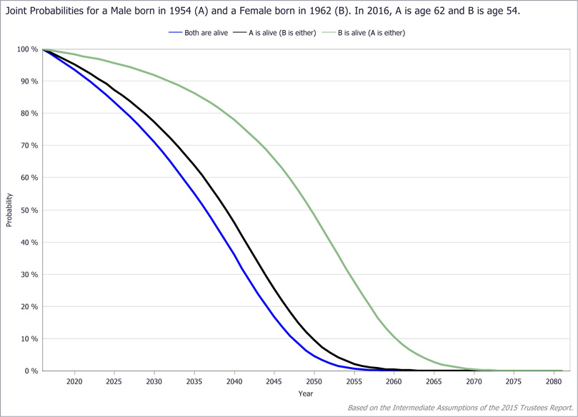
For benefit-claiming decisions, and retirement planning in general, married individuals have not only themselves to consider but, maybe more importantly, their spouses. The following examples of joint probability consider the male subject born in 1954 married to a woman born in 1962.5
Both Are Alive
Exhibit 12 plots the probability that both husband and wife are alive for each year from 2016 to 2081. Because the wife would be 119 in 2081, it is the last calendar year in which at least one of them could be alive. The survival functions for each individual are shown for comparison. The both-alive curve is necessarily lower than the survival curve for each individual, as it is always less likely that both will be alive than that either individual will survive alone. The probability of both being alive could be used to examine such questions as the likelihood that the couple's current income sources can support the two of them, or how long they should reasonably expect their current living arrangement to be appropriate before downsizing.
LV Joint Survivability tab: Sample query results (both are alive)
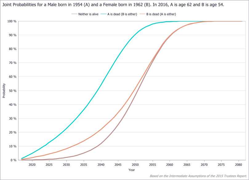
Both Are Dead
Exhibit 13 shows the converse to the situation in which both are alive: the probability that both are dead in a given year. This function could be useful for younger parents assessing the risk that neither will be alive to care for their dependent children. Similar to both being alive, the probability of both being dead is always less than that of either individual alone being dead. Note also that the complement of both being dead is the case of at least one alive, an important metric for longer-term planning.
LV Joint Survivability tab: Sample query results (both are dead)
Only One Is Alive
Cases in which one spouse survives alone may be more important for couples planning retirement strategies than are the cases of both spouses being alive or both being dead. Single-survivor cases are particularly relevant because one spouse is likely to outlive the other.
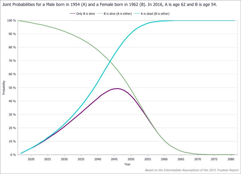
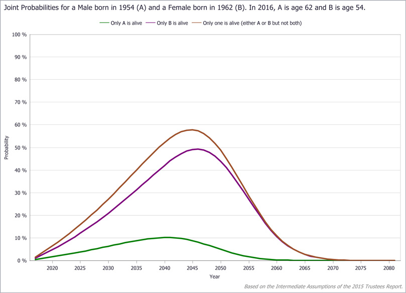
Exhibits 14 and 15 show the respective one-survivor probability curves for the subject couple. In contrast to the curves for both being alive and both being dead, which are essentially aggregate functions of survival, the curves for only one spouse surviving generally rise then fall as age advances. The initial rise is due to the decreasing chance that both will remain alive, or rather the increasing chance that one of the two will die, leaving the other as the sole survivor. The probability reaches a peak after which it begins to decline, which is due to the increasing likelihood that both will have died with the passage of time.
These probabilities are informative in many scenarios. For example, suppose our subject couple has no income besides the husband's earnings and is contemplating when to begin relying heavily on OASDI retirement benefits. Exhibit 14 shows the probability that the wife will outlive her husband and thus lose the income stream of his earnings. That scenario worries them, as the probability increases steadily and substantially to nearly 50 percent at its peak 30 years into the future.6 Although their ages differ by only 8 years, the wife has at least a 15 percent chance of being a widow by her mid-60s. If she reaches age 80, the chance rises to more than 45 percent.
The probability that the wife survives alone is the product of the probability that she is alive and the probability that the husband is dead. Exhibit 14 plots those two probabilities for the subject couple. Exhibit 15 shows the opposite situation—the husband is alive but the wife is dead—along with the probability that either one of them will be alive without the other, which is the sum of the two individual probabilities (see Appendix B). By visualizing the probabilities of the various scenarios, the couple can assess their situation in a broader context and make better-informed decisions.
LV Joint Survivability tab: Sample query results (only one is alive, specifying which spouse)
LV Joint Survivability tab: Sample query results (only one is alive, with and without specifying which spouse)
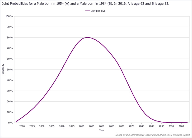
Another circumstance in which sole survivorship might be of great concern is that of a single parent caring for a dependent adult child. Suppose, for instance, the 62-year-old male subject has a 32-year-old disabled son. For this exercise, assume that the son's disability does not affect his survival function. With no earnings or appreciable assets of his own, the son is supported by his father's current earnings. The father's death would leave the son without the support necessary to continue the desired level of care. Exhibit 16 plots the probability that the son survives alone in each year from 2016 onward. Without some form of insurance in place to cover the cost of care for the rest of his son's life, the father views even a 5 percent probability that his son might be alive without him to be an unacceptable risk. That probability is exceeded in only 5 years (by 2021), and rises dramatically to 80 percent by 2053. To be prudent, the father promptly explores insurance, annuities, and other contingency plans in anticipation of his disabled son surviving him.
LV Joint Survivability tab: Sample query results (father is dead, son is alive)
Conclusion
The LV is a visual-analysis tool for exploring applications of the OCACT cohort life tables. Data in the life tables are presented as two basic series in the LV—survival functions and age-at-death probability distributions—each of which is generated for each potential age and each sex across a long range of historical and projected birth cohorts. The LV is designed to make the information contained in those life tables available in an accessible form to analysts, researchers, and others exploring such applications as financial and retirement planning, public policy analysis, and individual decision making that requires longevity projections. The analytic capabilities of the LV are also designed to stimulate research ideas in a highly interactive manner, with particular emphasis on data visualization. Future extensions to the LV will model a number of specific analytic problems that depend strongly on age-specific survival projections, such as the decision of when (and how) to claim Social Security benefits to maximize insurance value—especially for such cases as married couples whose crucial joint-survival probabilities are not otherwise easily obtained.
Appendix A: Computation of LV Functions
The LV expresses age in the format years:months, such that 65 years and 8 months is expressed 65:08. The LV assumes that no individuals survive to age 120. Although this is not completely true, it is more than sufficient for all practical purposes. Thus, anyone alive at age 119:11 will die within a month and no one will ever be alive at age 120:00.
In the LV there are two primary functions computed from (the probability that an individual aged years will die within 1 year). The survival function is the probability that an individual aged will attain age . The probability density function of death is the probability of death during each successive age for a population at initial age . From the and functions, other values and functions are easily derived, such as survival-age quantiles and the chances of survival beyond a given age. For instance, the age before which 95 percent of a population at initial age will die is also the age beyond which 5 percent of that population will survive, with both values computed from .
Assuming an initial 100 percent population for each cohort at birth, or , the surviving fraction of that population at the beginning of each successive annual age is calculated as for all ages from 1 to 120. Because and , the function can be used to derive the probability of death during each annual age of the cohort simply as .
Because many OASDI program rules specify monthly rather than yearly intervals (such as the benefit payment schedule and the formula for adjusting the benefit amount by claiming age), the annual mortality data in the life tables are converted to monthly equivalents before any functions are calculated. Although other actuarial methods can provide a more accurate monthly interpolation of the annual mortality rates, an assumed uniform distribution of death within each annual age is sufficient for the LV's intended users.7 Thus, the probability of death during each month within an annual age is calculated simply as the respective annual probability divided by 12. Further calculations no longer need the original annual data, so can now refer exclusively to a specific monthly age. The survival function from birth (), initially 1, is now recomputed for each successive monthly age from 1 to 1,440 months (120 years) simply as .
With the monthly and functions fully computed from birth through 1,440 months, the final calculations are the age-specific and functions; that is, for a population alive at a given initial monthly age , and are computed from that initial age forward through month 1,440. Thus, the survival function and the death probability function for each monthly age from 1 to 1,440 and for each monthly age from to 1,440.
Appendix B: Joint Probability Calculations
Listed below are the equations for all possible probabilities of joint survival for two persons, and . The notation denotes the probability of person being alive at a given future point, and the probability of having died by that time is thus . For person , the respective notations are and . Each person's survival is assumed to be independent of the other's.
- Both persons are alive.
- A is alive and B is dead.
- B is alive and A is dead.
- Both A and B are dead.
- Only one is alive (Only A or Only B, but not Both).
- At least one person is alive (Only A, Only B, or Both).
Note that the universe is composed of the probabilities Both, Only A, Only B, and Neither, which sum to 1.
Notes
1 The 2015 Trustees Report is available at https://www.socialsecurity.gov/oact/TR/2015/index.html; section V.A2 discusses the mortality assumptions it employs. Each year, OCACT develops three independent estimates of the future mortality rates, comprising an intermediate scenario (its “best guess”), a low-cost scenario, and a high-cost scenario. In the low-cost scenario, the cohort populations essentially die off more quickly than they do in the intermediate case, resulting in a comparatively smaller beneficiary population and reduced Social Security outlays. In the high-cost scenario, the cohort populations die off more slowly, resulting in more beneficiaries and increased outlays. The intermediate-scenario projections are the basis of most Social Security policy discussions and reform proposals.
2 The life tables do not include figures for combined-sex populations.
3 Data in cohort life tables are averages for the population in question. Of course, many people live much longer or shorter than their life expectancies, and their actual survival functions can be radically different from those in the tables given their health, lifestyle, genetics, and other factors. Those who expect to live longer than average could benefit from delayed claiming, if they can afford to do so.
4 The joint probability computations in the current version of the LV are limited to two persons. In future versions, the computations will be extended to include three or more persons.
5 In a joint-probability analysis between two or more persons it is preferable to include relevant data (such as life tables) on their prevailing joint condition or relationship (such as a married couple, parents and their children, or business partners in a given industry or occupation). In the absence of such data, the joint-probability computations presented here suffice if one can accept complete independence of survival of the two persons.
6 Note that these values reflect the probabilities of a death event occurring as of the given year rather than in that given year.
7 For the definition of a variable that also assumes a uniform distribution of death within each age beyond the birth year, see Bell and Miller (2005, 4–5).
References
Bell, Felicitie C., and Michael L. Miller. 2005. Life Tables for the United States Social Security Area 1900–2100. Actuarial Study No. 120. SSA Pub. No. 11-11536. Baltimore, MD: Social Security Administration, Office of the Chief Actuary. https://www.socialsecurity.gov/OACT/NOTES/pdf_studies/study120.pdf.
Meyer, William, and William Reichenstein. 2010. “Social Security: When Should You Start Benefits and How to Minimize Longevity Risk?” Journal of Financial Planning 23(3): 52–63.