The Economic Consequences of a Husband's Death: Evidence from the HRS and AHEAD
Social Security Bulletin, Vol. 65, No. 3, 2003/2004 (released January 2005)
Despite increased labor force participation rates among women and reforms under the Employee Retirement Income Security Act, widowhood remains an important risk factor for transition into poverty, although somewhat less so than 20 years ago. Women widowed at younger ages are at greatest risk for economic hardship after widowhood, and their situation declines with the duration of widowhood. We also find that women in households that are least prepared financially for widowhood are at greatest risk of a husband's death, because of the strong relationship between mortality and wealth.
Purvi Sevak is an Assistant Professor of Economics in the Department of Economics, Hunter College, City University of New York; David R. Weir is Research Professor and Associate Director of the Survey Research Center of the Institute for Social Research and Assistant Director of the Health and Retirement Study at the University of Michigan; and Robert J. Willis is Professor of Economics and Research Professor in the Survey Research Center and the Population Studies Center of the Institute for Social Research and the Principal Investigator for the Health and Retirement Study at the University of Michigan.
Acknowledgments: This work was supported by a grant from the Social Security Administration through the Michigan Retirement Research Center (Grant No. 10-P-98358-5). The findings and conclusions are solely those of the authors and should not be considered as representing the views of the Social Security Administration or any agency of the federal government. This article was previously published by the University of Michigan Retirement Research Center, Ann Arbor, as "The Economic Consequences of Widowhood," Working Paper WP 2002-023, April 2002, under the project "The Impact of Widowhood on the Economic Status of Women," Project No. UM99-05.
Contents of this publication are not copyrighted; any items may be reprinted, but citation of the Social Security Bulletin as the source is requested. The findings and conclusions presented in the Bulletin are those of the authors and do not necessarily represent the views of the Social Security Administration.
Summary
Households headed by elderly women still experience substantially higher rates of poverty than do other households. In this article, we use longitudinal data from the Health and Retirement Study to examine why widowed women are so much more likely than married women to have poor economic status, when they themselves were once married. We examine whether high rates of poverty are due to income lost upon a husband's death, to depletion of assets, or to selection effects. Although we find that widowhood does increase the incidence of poverty among women who were not poor when married, the substantial number of widows in poverty reflects poor economic status that continued from marriage to widowhood. Poor women are more likely to become widowed at a young age, because of the relationship between mortality and socioeconomic status.
The findings in this article provide a brighter outlook for widows than do studies of widows in earlier decades. In the 1970s, 37 percent of new widows became poor after widowhood. By the 1990s, this rate had fallen to between 12 percent and 15 percent. Nevertheless, widowhood remains an important risk factor for transition into poverty. Faced with the loss of resources in widowhood, women have only a few options available to improve their economic status. Remarriage is difficult because of the demographic imbalances caused by shorter male life expectancy. We find some evidence that widows live with children or siblings so that they can be part of a household with more resources. Although earning income through work is the main way women can improve their status, it becomes increasingly difficult to achieve with age, and we cite little evidence of it in our article.
Women who are least able to prepare for widowhood and therefore are at greatest risk of widowhood, because of the relationship between mortality and wealth, give cause for Social Security policy to remain attentive to the special situation of widows. We would suggest that additional attention be paid to the welfare of women widowed after their children have grown but before they have completed their retirement preparations. These women are generally not eligible for Temporary Assistance for Needy Families, Supplemental Security Income, or Social Security and thus are most vulnerable to poverty. Even women who have some accumulated wealth are more likely to be in poverty many years later, as they are forced to spend down their wealth in the years before gaining Social Security eligibility.
Introduction
High rates of poverty among widows, especially those living alone, remain a primary concern of policies for the elderly (Burkhauser 1994; Sandell and Iams 1997). Expansion of Social Security and Supplemental Security Income, women's increasing educational attainment and labor force participation rates, and changes in policies regulating employer-provided pension plans should have improved the economic status of women during the past few decades. Nevertheless, households headed by elderly women still experience substantially higher rates of poverty than do other households. In this article, we use the Health and Retirement Study (HRS) to examine the economic status of older, widowed women in the 1990s.
Several main determinants of a widow's economic status have been discussed in the literature (Zick and Smith 1991), such as economic preparedness of intact married couples for potential widowhood, expenses associated with a husband's death, and declining economic status associated with the duration of widowhood. We evaluated the first component in previous work, using the baseline 1992 wave of the Health and Retirement Study (Weir and Willis 2000). Using measures of full wealth (defined here as financial assets plus pensions and Social Security) of married couples and the amount of full wealth that would remain for a widow if the husband died immediately following the interview date, we found considerable variation in the provision for widows, holding constant the resources of the marriage.
This article tackles the first and third components of the economic status of widows using income and wealth data from the cross-sectional and the longitudinal aspects of the HRS and the study of Asset and Health Dynamics Among the Oldest Old (AHEAD). We also examine a fourth determinant of economic status: selection effects that make widowhood more likely for women who have fewer economic resources. We find that one of the reasons poverty rates among widows are substantially higher than poverty rates among married women is that poorer married women are more likely to become widowed.
In this article, we
- discuss the HRS data;
- compare measures in the HRS to those in the Current Population Survey (CPS), which has been the primary data set used to study poverty among the elderly;
- examine how assets and different components of income change over time among women with different marital status changes;
- attempt to disentangle the relationship between higher rates of poverty and duration of widowhood; and
- study the relationship between income and mortality risk to assess the extent to which high rates of poverty among widows are due to selection effects.
Data
The data used in this article are from the 1992 to 1998 waves of the Health and Retirement Study. The HRS merged two data sets: the original HRS, which first collected data in 1992 on individuals born between 1931 and 1941, and the AHEAD study, which first collected data in 1993 on individuals born before 1924. In 1998, the two original studies were combined, and two new cohorts were added to produce a cross-sectional sample that is representative of the U.S. population born in the years up to 1947 (that is, people aged 51 or older in 1998).
Much of the existing literature on elderly poverty uses data from the March Current Population Survey. Pooled cross sections of the CPS can be used to track trends over time, since the CPS has been collected annually for many years and the survey measures have not changed much from year to year. One of the goals of this article is to illustrate how the HRS can add to the study of poverty and to other measures of economic well-being among elderly households undergoing transitions in family structure.
Unlike the CPS, the HRS reinterviews its sample members every 2 years until the respondent's death. Thus, a longitudinal data set can be constructed to directly examine whether and why widowhood is associated with higher rates of poverty and how economic status evolves over the duration of widowhood. The 1998 wave plus the first two waves (1992 and 1994) of the original HRS (that is, persons born between 1931 and 1941) and the first two waves (1993 and 1995) of the AHEAD study (persons born before 1924) are combined to conduct the longitudinal analyses in this article. The full 1998 sample of individuals aged 51 and older is used to present the cross-sectional analyses for 1998.
The HRS elicits detailed information on assets, pensions, housing, insurance, and Social Security eligibility, in addition to information about income. Other studies of widowhood have had to focus more narrowly on current income, thereby neglecting the full potential to support lifetime consumption and often producing the appearance of volatile movements into and out of poverty (Bound and others 1991; McGarry 1995). The HRS can be used to replicate conventional income-based definitions of poverty, but it can also be used to study the long-term implications of changes in marital status on wealth. In the next section, we replicate CPS-based measures of poverty with the HRS to assess whether measures in the HRS are comparable with those in the CPS.
Widows' Wealth, Income, and Poverty, 1992–1998
HRS and AHEAD poverty rates among women for selected years are compared with CPS rates in Tables 1 and 2. Overall, estimates of poverty from the HRS 1998 cross section are slightly lower than similar estimates from the CPS (10.9 percent vs. 12.2 percent for all women) in Table 1. This is most likely due to slight improvements in the HRS survey design compared with the design of the CPS. For example, missing data are a perennial problem for which the HRS uses a series of structured questions called unfolding brackets to identify a range for the true value and greatly reduce the error from imputations. Thus, respondents in the HRS may more fully report their income from different sources. An additional difference between the studies is that the HRS treats unmarried couples who report they live together "as if married" as a single financial unit, thereby combining the incomes of both partners. The CPS, however, does not indicate whether two unrelated people have a shared financial relationship. Still, since the gap between the poverty estimates exists even for married women, this is not likely to be the sole factor driving the different estimates.1
| Age in survey year | All women in survey |
Married | Divorced or separated |
Widowed | Never married |
|---|---|---|---|---|---|
| Health and Retirement Study | |||||
| All | 10.9 | 3.9 | 19.7 | 17.3 | 26.2 |
| 51–64 | 9.4 | 4.5 | 16.5 | 19.6 | 22.3 |
| 65–79 | 10.3 | 2.8 | 26.0 | 14.5 | 26.6 |
| 80 or older | 19.0 | 4.0 | 33.3 | 20.3 | 41.1 |
| Current Population Survey | |||||
| All | 12.2 | 5.6 | 22.1 | 18.6 | 21.4 |
| 51–64 | 11.0 | 5.5 | 21.5 | 21.4 | 22.8 |
| 65–79 | 12.2 | 5.5 | 23.9 | 17.2 | 21.5 |
| 80 or older | 16.6 | 7.5 | 21.0 | 19.1 | 16.2 |
| SOURCE: Author's calculations using data from 1998 from the Health and Retirement Study and the Current Population Survey. | |||||
| Survey year | Age | All women in survey |
Married | Divorced or separated |
Widowed | Never married |
|---|---|---|---|---|---|---|
| Health and Retirement Study Panel, 1992–1998 | ||||||
| 1992 | 51–61 | 10.3 | 4.9 | 21.6 | 21.5 | 21.1 |
| 1994 | 53–63 | 11.6 | 4.8 | 23.6 | 26.5 | 26.5 |
| 1998 | 57–67 | 10.4 | 4.2 | 20.2 | 19.7 | 26.9 |
| Current Population Survey Pseudo-Panel, 1992–1998 | ||||||
| 1992 | 51–61 | 11.2 | 6.1 | 21.9 | 25.3 | 19.9 |
| 1994 | 53–63 | 11.7 | 6.4 | 21.7 | 24.8 | 22.0 |
| 1998 | 57–67 | 12.2 | 6.4 | 23.1 | 21.6 | 25.5 |
| Asset and Health Dynamics Among the Oldest Old Panel, 1993–1998 | ||||||
| 1993 | 70 or older | 15.8 | 6.1 | 29.3 | 20.1 | 24.2 |
| 1995 | 72 or older | 14.2 | 4.4 | 26.9 | 18.3 | 21.9 |
| 1998 | 75 or older | 14.4 | 2.7 | 27.2 | 17.8 | 31.3 |
| Current Population Survey Pseudo-Panel, 1993–1998 | ||||||
| 1993 | 70 or older | 17.5 | 7.6 | 27.6 | 22.0 | 26.3 |
| 1995 | 72 or older | 17.0 | 7.3 | 29.1 | 20.3 | 29.7 |
| 1998 | 75 or older | 15.0 | 6.1 | 25.0 | 18.3 | 20.2 |
| SOURCE: Author's calculations using data from 1992, 1994, and 1998 of the Health and Retirement Study and from 1992, 1994, and 1998 of the Current Population Survey and from 1993, 1995, and 1998 of the Asset and Health Dynamics Among the Oldest Old study and from 1993, 1995, and 1998 of the Current Population Survey. | ||||||
Both data sources show the enormous differential in poverty rates between married and unmarried women. In the 1998 HRS, just less than 4 percent of all married women were impoverished compared with 17 percent of widowed women (Table 1). This differential exists across birth cohorts, as well as in all waves of both data sets. In Table 1, the data also show that poverty rates increase with age. This can most clearly be seen in the top panel, with poverty rates by age pooled across all marital groups. However, this pattern of poverty rates increasing with age does not exist consistently within marital status categories, suggesting that most of the overall trend is due to the fact that the percentage of women with husbands declines with age.
In recent years, the economic status of widows has improved relative to other nonmarried women, as shown in their lower poverty rates when compared with the rates of divorced or never-married women in most of our comparison periods (Tables 1 and 2). This may be due to the Employee Retirement Income Security Act (ERISA) pension reforms of 1974 and the Retirement Equity Act (REA) of 1984. ERISA changed the default payout option for pensions from a single-life benefit to a joint-and-survivor benefit. Under a single-life benefit, households lose all pension annuity payments upon the death of the spouse whose job provided the pension, whereas a joint-and-survivor benefit continues annuity payments to the surviving spouse. Until REA in 1984, the worker was still allowed to choose a single-life benefit. The REA amended ERISA to require the spouse's signature if a worker wants to select the single-life benefit, instead of the default joint-and-survivor option. These changes since 1974 have substantially increased the percentage of widows who receive a survivor pension (Holden and Nicholson 1998).
Next, the trends in pension income are analyzed in relation to three other components of income that may be affected by marital transitions: earned income, Social Security, and the income of family members in the same household. Although poverty measures take into account only income and family size, trends in asset levels are also examined because the overall economic status of widows is determined by assets as well. In each case, trends between baseline (1992 for HRS, 1993 for AHEAD) and 1998 data, in 1998 dollars, are compared. Three groups are shown: women who were married throughout the interval (married or continually married), women who became widowed during the interval (new widows), and women who were widowed throughout the interval (widows or continually or existing widows). The goal of this analysis is to compare the trajectory of new widows with those of existing widows and continually married women.
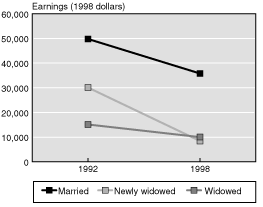
Family earnings in 1992 and 1998 among these three groups of women in the HRS are plotted in Chart 1. Average earnings decline for all three groups over this period, partly because families in the HRS are retiring during this period. Mean family earnings for continuously married households declined by about 30 percent, from $50,000 to $35,000, and by a similar percentage for households with existing widows, from about $15,000 to $10,000. Not surprisingly, the drop in household family earnings for new widows was much more dramatic, with earnings falling by more than 300 percent, from about $30,000 to less than $10,000.
Changes in mean family earnings of HRS women from 1992 to 1998, by marital status
| Year | Married | Newly widowed |
Widowed |
|---|---|---|---|
| 1992 | 49,757 | 30,077 | 15,129 |
| 1998 | 35,801 | 8,471 | 10,026 |
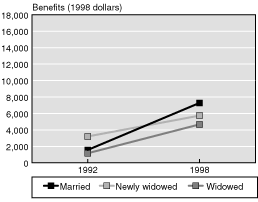
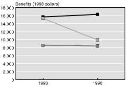
Changes in household Social Security benefits for the same groups are shown in Chart 2, for the HRS and the AHEAD study. The patterns among the AHEAD cohort in the bottom panel of Chart 2 reflect perfectly the rules of the Social Security system, in which benefits are based on lifetime earnings and adjust by formula after widowhood. New widows in the AHEAD study had nearly the same benefits as those of married women in 1993, suggesting that new widows had similar lifetime incomes. Following a husband's death, widow benefits will in general range from 67 percent of the married level, assuming the spousal benefit was equal to half that of the primary earner, down to 50 percent replacement in the case in which both partners had equal benefits based on earnings. New widows averaged about $10,000 per year in benefits in 1998 compared with just over $15,000 when married (1993), indicating that nearly all of them had benefits that were based on their husband's earnings record. Continuously married and continuously widowed households showed essentially no change. Since poverty thresholds are based on equivalence scales for family size, this adjustment in benefits contributes little to differences in poverty rates.
Changes in Social Security benefits of HRS women and AHEAD women, by marital status
| Year | Married | Newly widowed |
Widowed |
|---|---|---|---|
| HRS women, 1992 and 1998 | |||
| 1992 | 1,576 | 3,212 | 1,170 |
| 1998 | 7,285 | 5,743 | 4,675 |
| AHEAD women, 1993 and 1998 | |||
| 1993 | 15,663 | 15,300 | 8,576 |
| 1998 | 16,300 | 9,903 | 8,408 |
In the HRS cohort, the patterns are primarily determined by who claims benefits and who does not (Chart 2, top panel). The median age of the HRS cohort, which ranged in age from 51 to 61 in 1992, was only 56 in 1998, so none of the cohort was eligible to claim benefits in 1992 and roughly half the cohort was not eligible to claim retirement benefits in 1998. Women in families receiving benefits in 1992 were thus married to older men. Families of new widows were more likely to be receiving benefits while married in 1992, because their husbands were older and partly because their husbands may have been more likely to collect early retirement benefits (at age 62) on the basis of poorer health. After widowhood, these new widows had higher average benefits than they did at baseline, because many of them became eligible to claim benefits between 1992 and 1998. Continuously married women experienced the greatest growth in mean benefits received, because they were less likely than the others to be receiving benefits in 1992 and because they were entitled to higher benefits when claimed.
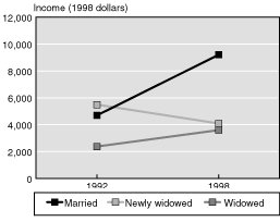
Income from pension and annuities, illustrated in Chart 3, drops for new widows in the HRS and the AHEAD study. In contrast, existing widows and continuously married women both were the beneficiaries of increased pension and annuity income in the HRS and AHEAD. This growth for stable marriages and continuing widows in the AHEAD study suggests that some of the income may be based on funds whose payout depends on equity values, which improved over this time period. In both studies, the gap between new widows and the continuously married in 1998 was on the order of $5,000 per year. It is somewhat surprising that pension income among new widows in HRS should decline, because many men had not yet claimed pension income. It appears, however, that among married men at baseline, those who would eventually leave a widow were more likely to have taken early retirement, perhaps because of poor health, and in both cohorts pension benefits were reduced after death.
Changes in pension and annuity income of HRS women and AHEAD women, by marital status
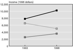
| Year | Married | Newly widowed |
Widowed |
|---|---|---|---|
| HRS women, 1992 and 1998 | |||
| 1992 | 4,693 | 5,498 | 2,376 |
| 1998 | 9,206 | 4,093 | 3,600 |
| AHEAD women, 1993 and 1998 | |||
| 1993 | 7,813 | 6,555 | 2,537 |
| 1998 | 10,214 | 5,020 | 3,569 |
These steep declines in pension income for new widows may be surprising given the ERISA and REA reforms that require both spouses' signatures to claim pension benefits on a single-life annuity. However, joint-and-survivor annuities that provide only 50 percent of survivor benefits are a common default plan that does not require the potential survivor's signature. Thus, while total loss of pension benefits after a husband's death has become uncommon, full retention is also rare.
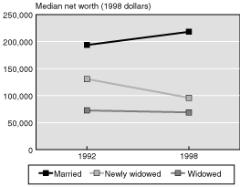
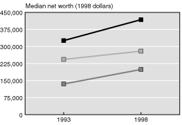
Because of the relative loss in income among new widows, those women might be expected to draw down on their wealth at a faster rate than others.2 This would be especially true among nonelderly new widows who are too young to get Social Security benefits. The course of median net worth for women in the HRS (aged 51 to 61) and AHEAD study (aged 70 or older), is shown in Chart 4, top panel and bottom panel, respectively. Women who are about to become widowed start out with lower levels of wealth compared with women whose marriages will continue, which is consistent with recent findings in Zick and Holden (2000). In both cohorts, continuing widows made essentially no gains during a boom market, while continually married women showed further increases in wealth. In addition to new widows drawing down wealth more rapidly, this difference in net worth between married women and widows also reflects the fact that a smaller portion of the assets of widows are held either directly or indirectly in equities. The main contrast between new widows in the two age groups is the difference in net worth: new widows in the HRS lost enough wealth to fall nearly to the level of continuing widows by 1998; new widows in the AHEAD study posted gains in net worth. One possible explanation of this pattern is that younger widows (aged 51 to 61) consume their assets at a greater rate because they are not yet eligible for Social Security.
Changes in median net worth of HRS women and AHEAD women, by marital status
| Year | Married | Newly widowed |
Widowed |
|---|---|---|---|
| HRS women, 1992 and 1998 | |||
| 1992 | 193,563 | 130,625 | 72,438 |
| 1998 | 218,000 | 96,000 | 69,000 |
| AHEAD women, 1993 and 1998 | |||
| 1993 | 325,748 | 242,894 | 134,873 |
| 1998 | 417,862 | 279,335 | 198,778 |
This comparison of income and assets between continuing wives, continuing widows, and new widows shows relative declines after widowhood for several components of income. In the HRS, family earnings for preretirement new widows decline faster than they do for women whose husbands remain alive (Chart 1). Pension and annuity income declines for younger (aged 51 to 61) and older (aged 70 or older) new widows (Chart 3). Social Security benefits increase at a slower rate for young new widows than for other women (married women or existing widows), perhaps because husbands of new widows were more likely to have claimed early benefits (Chart 2, top panel). Among older existing widows, there are no changes in Social Security that would increase poverty (Chart 2, bottom panel).
Duration Effects on Widow Poverty
The comparison of the positions of new widows, continuing widows, and married women between baseline (1992 HRS, 1993 AHEAD) and 1998 HRS suggests that the economic status of widows and married women may diverge with the duration of widowhood. The net worth of women widowed at baseline grows at a much slower rate than that of married women (Chart 4);3 pension and annuity income among continuing widows also increases at a slower rate than it does among married women (Charts 4 and 5), and the women who were widowed early (before baseline as opposed to since baseline) are worst off financially across all measures.
Duration of widowhood could be related to economic status in a number of ways. First, if a couple has not adequately planned for widowhood, the economic status of the widow may decline with the length of time that she is widowed. Second, widows may make economic adjustments, such as reentering the workforce, selling a home, or living with others, which may improve their economic status over time. Third, duration effects could reflect selection into widowhood.
Those who have been widowed longest are more likely to have become widowed at a younger age. The well-documented correlation between wealth and health (Smith 1999) is one of the mechanisms driving the selection of women into widowhood. Poorer husbands have a lower life expectancy than do their wealthier peers; women married to poorer men will thus be widowed at an earlier age and will make up a disproportionate share of widows and especially of long-duration widows. Lower baseline levels of wealth of new and existing widows, in 1992 and 1993, in Chart 4 are consistent with this selection. In this section we examine further the evidence of widow duration on poverty rates.
The Health and Retirement Study obtains retrospective marital history information from all respondents at baseline, with which the date when women most recently became widowed, and thus the length of time they have been widowed, can be calculated for all widows present in 1998. Poverty rates among widows vary by age and by duration of widowhood (Chart 5). A U-shaped pattern emerges when analyzing the effects of age: poverty rates are high for widows under the age of 65, substantially lower for widows aged 65 to about 80, and then high again among the oldest old. In general, duration effects portray more of a J-shaped pattern: starting high at very short durations, dropping lower for the next 10 years, and then rising rapidly at longer durations. The short durations are problematic (see also Burkhauser and others 1986). By the nature of the HRS interview, income earned by the deceased husband will not be reported, even if he was alive for part of the preceding calendar year, and some of these women have not yet received the adjustments to Social Security or pension survivor benefits that will eventually raise their incomes.
Poverty rates of widows, by age and duration of widowhood
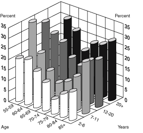
| Age | 2–6 years | 7–11 years | 12–20 years | 20+ years |
|---|---|---|---|---|
| 55–59 | 20.3 | 34.4 | 31.3 | . . . |
| 60–64 | 21.4 | 21.2 | 27.3 | 31.1 |
| 65–69 | 17.3 | 14.4 | 24.9 | 27.0 |
| 70–74 | 13.5 | 10.1 | 18.9 | 19.0 |
| 75–79 | 7.0 | 12.3 | 16.7 | 24.0 |
| 80–84 | 11.0 | 16.1 | 20.6 | 25.0 |
| 85+ | 13.5 | 24.6 | 22.6 | 28.1 |
| NOTE: . . . = not applicable. | ||||
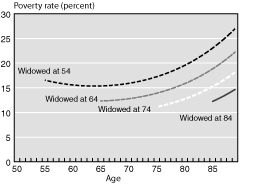
The statistical association between poverty and duration of widowhood is clear, excluding short durations: the greater the duration, the greater the risk of being in poverty. In an analysis of variance, the duration categories explain about twice as much of the variance as do the age categories. Regression analysis can be used to generate synthetic profiles of the risk of poverty as a function of age and duration. The predicted probability of poverty is obtained by regressing whether or not a woman is in poverty on the categories of age at and duration of widowhood. The simulated profiles in Chart 6, estimated from a single cross section and not from true longitudinal observations, suggest that more than 15 percent of women widowed at the age of 54, before they are eligible for Social Security retirement income, will be in poverty upon the death of their husband. Poverty rates of widows decline initially, up to about the age of 65, most likely because of the receipt of Social Security benefits, and then rates increase systematically as widows age, with poverty rates of 20 percent or higher occurring once they reach their 80s. Women widowed at the age of 64 or 74 have lower initial poverty rates, but their economic position deteriorates steadily as well. At any given age, the women who had been widowed longest (that is, at the youngest ages) had the higher poverty rates.
Predicted probability of poverty of widows, by age at widowhood and duration of widowhood
| Age | Widowed at 54 | Widowed at 64 | Widowed at 74 | Widowed at 84 |
|---|---|---|---|---|
| 55 | 16.5 | . . . | . . . | . . . |
| 56 | 16.3 | . . . | . . . | . . . |
| 57 | 16.1 | . . . | . . . | . . . |
| 58 | 15.9 | . . . | . . . | . . . |
| 59 | 15.7 | . . . | . . . | . . . |
| 60 | 15.6 | . . . | . . . | . . . |
| 61 | 15.5 | . . . | . . . | . . . |
| 62 | 15.4 | . . . | . . . | . . . |
| 63 | 15.4 | . . . | . . . | . . . |
| 64 | 15.3 | . . . | . . . | . . . |
| 65 | 15.4 | 12.3 | . . . | . . . |
| 66 | 15.4 | 12.4 | . . . | . . . |
| 67 | 15.5 | 12.4 | . . . | . . . |
| 68 | 15.6 | 12.5 | . . . | . . . |
| 69 | 15.7 | 12.6 | . . . | . . . |
| 70 | 15.9 | 12.8 | . . . | . . . |
| 71 | 16.1 | 13.0 | . . . | . . . |
| 72 | 16.3 | 13.1 | . . . | . . . |
| 73 | 16.6 | 13.4 | . . . | . . . |
| 74 | 16.9 | 13.6 | . . . | . . . |
| 75 | 17.2 | 13.9 | 11.2 | . . . |
| 76 | 17.6 | 14.2 | 11.4 | . . . |
| 77 | 18.0 | 14.6 | 11.7 | . . . |
| 78 | 18.5 | 15.0 | 12.0 | . . . |
| 79 | 19.0 | 15.3 | 12.3 | . . . |
| 80 | 19.5 | 15.8 | 12.7 | . . . |
| 81 | 20.1 | 16.3 | 13.2 | . . . |
| 82 | 20.8 | 16.9 | 13.6 | . . . |
| 83 | 21.5 | 17.5 | 14.1 | . . . |
| 84 | 22.2 | 18.1 | 14.7 | . . . |
| 85 | 23.0 | 18.8 | 15.2 | 12.2 |
| 86 | 23.9 | 19.6 | 15.9 | 12.8 |
| 87 | 24.9 | 20.4 | 16.6 | 13.4 |
| 88 | 25.9 | 21.2 | 17.3 | 14.0 |
| 89 | 27.0 | 22.2 | 18.1 | 14.7 |
| NOTE: . . . = not applicable. | ||||
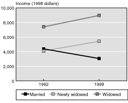
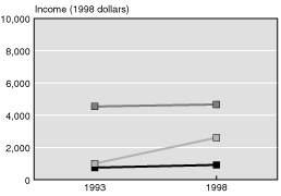
One way in which widows at any age can compensate for reduced economic status is to live with other family members. Not much is known about the allocation of resources within such multigenerational households. The poverty scales assume that income is pooled and treat coresident family members as a single economic unit. In Chart 7, changes in other-person income are followed for the three marital transition groups: continuously married women, new widows, and continuing widows. Continuously married women have very little other-person (nonspousal) income. In HRS, their average level declines over time because of the departure of young adult children from some households (Chart 7, top panel). Existing widows at baseline, however, had much higher levels. In HRS and AHEAD, newly widowed women increased their other-person income by about $1,500. By 1998, they had substantially more than continuously married women but still less than continuously widowed women (Chart 7). This could reflect either a slow adjustment process for new widows or a worse personal economic situation for women widowed earlier. In the HRS cohort, where the difference between new and continuing widows in 1998 was very large, it almost certainly reflects lower personal resources of early widows who in the past moved in with other family members.
Changes in income of other family members of HRS women and AHEAD women, by marital status
| Year | Married | Newly widowed |
Widowed |
|---|---|---|---|
| HRS women, 1992 and 1998 | |||
| 1992 | 4,376 | 4,088 | 7,402 |
| 1998 | 3,057 | 5,419 | 8,957 |
| AHEAD women, 1993 and 1998 | |||
| 1993 | 748 | 1,000 | 4,538 |
| 1998 | 916 | 2,604 | 4,662 |
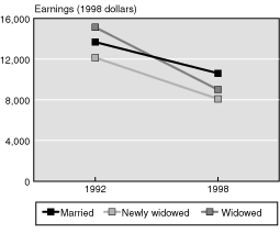
A second response mechanism is earnings from work, which is analyzed for the HRS cohort only in Charts 1 and 8. In Chart 1, mean family earnings for the three marital transition groups decline over time, as some of the cohort retires, but the decline for new widows is larger than it is for the others. From this chart, it is not clear how much of the decline was due to lost husband's income and how much was due to changes in the woman's earnings. In Chart 8, the analysis of earnings information is for women only and shows that all women had earnings declines, with new widows consistently having lower earnings levels. By subtracting women's earnings from family earnings, the analysis shows that at baseline the men whose marriages remained intact earned about $36,000, compared with only $18,000 for men who would leave behind a widow by 1998. Earnings response was therefore not a significant factor in improving a widow's economic position, even in a cohort aged 57 to 67 at the end of the observation period.
Changes in earnings from work of HRS women from 1992 to 1998, by marital status
| Year | Married | Newly widowed | Widowed |
|---|---|---|---|
| 1992 | 13,677 | 12,148 | 15,129 |
| 1998 | 10,610 | 8,090 | 9,000 |
The strong statistical association between poverty and duration of widowhood could reflect any number of causal influences. Current age is exactly equal to age at widowhood plus duration of widowhood, and no statistical method can correctly identify the separate effects of all three. In Charts 5 and 6, which examine the relationship between duration and poverty by age, duration of widowhood is negatively correlated perfectly with age at widowhood. Women with the longest durations of widowhood were youngest when they became widows. Age at widowhood is likely to be important because of the life-cycle pattern of saving and dissaving for retirement and public programs. First, losing a husband before retirement incurs a loss of potential future private savings, pension accrual, and Social Security benefit increases. Consumption must be supported for several or many years before pension or Social Security benefits begin. In comparison, married women may be well prepared for widowhood in later life. Second, the death of a spouse is often associated with high medical expenses, more of which may be out-of-pocket expenses when death occurs, before Medicare eligibility begins at the age of 65. For these cohorts, the date of widowhood may also matter, given the reforms of ERISA in 1974 and REA in 1984.
Duration of widowhood is a proxy as well for the effects of several selection mechanisms that operate over time. Mortality rates are likely to be higher for poor women, leaving a smaller proportion of poor women as duration increases. Alternatively, if better-off widows are more likely to remarry, then we would expect to find increasing poverty with duration of widowhood. In the aggregate, poverty and duration of widowhood are positively correlated. However, another mechanism is likely to be at play, because remarriage selection is unlikely to dominate mortality selection. Among widows at wave 1 of HRS, 17 died and 6 remarried by wave 2. Among widows in AHEAD, 286 died and 8 remarried.
Duration of widowhood could also have a direct effect on particular sources of income. Social Security, which is adjusted for inflation at the same rate as that of the poverty thresholds, should not be affected by duration of widowhood. However, private pensions are not always indexed, and survivor benefits may not always be for the life of the widow, so it is possible that income from private pensions decreases with duration of widowhood. Finally, if private savings are consumed too quickly early in widowhood, less asset income will be available later in widowhood.
Crude descriptive evidence, then, indicates that current age and duration of widowhood are separately and independently related to poverty rates of widows. Because current age minus duration of widowhood equals the age at which widowhood began, we cannot infer from our data whether this pattern arises from true duration effects, such as overconsumption of assets, or from effects resulting from age at widowhood, such as greater shocks to lifetime income or stronger income-related selection effects at younger ages. The fact that the age profile of recent widows shows higher poverty rates at younger ages suggests that a woman's age at widowhood may primarily be driving the effects by duration. This selection into widowhood is examined in the next section.
Selection Effects on Poverty Among Widows
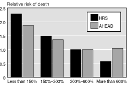
We first look at the correlation between mortality and socioeconomic status and examine whether, having controlled for age, a married man's probability of death is correlated with income. Using married couples at baseline (1992 or 1993), we estimate separate logistic regressions of the probability of a husband's death between baseline and 1998, as a function of the husband's age and of family income as a percentage of poverty. The relative risk of a husband's death varies as a function of household income relative to the poverty line (Chart 9). The relative risks were computed separately for each cohort, thus neutralizing the much higher average death rate in the older cohorts. The younger HRS cohort shows a somewhat steeper and more regular path of declining mortality with higher income. Couples with income less than 150 percent of the poverty line were 2.3 times more likely than the reference group (300 percent to 600 percent of poverty) to experience a husband's death. The AHEAD cohort shows similar but smaller differences by income: the group with income less than 150 percent of poverty was 1.8 times more likely to experience a husband's death. The highest income group in the HRS experienced only 60 percent of the deaths that the reference group did; in AHEAD, essentially no difference was present between the top group and the reference group.
Relative risk of husband's death, by family income as a percentage of poverty
| Income as a percentage of poverty level | HRS | AHEAD |
|---|---|---|
| Less than 150 percent | 2.29 | 1.87 |
| 150–300 percent | 1.49 | 1.36 |
| 300–600 percent | 1.00 | 1.00 |
| More than 600 percent | 0.57 | 1.04 |
| NOTE: Values reflect risk relative to that for the reference group (300 percent to 600 percent of poverty level income). | ||
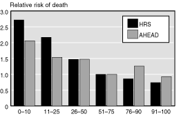
Because the income distributions differ between HRS and AHEAD, the logistic regressions were reestimated using percentile ranking in the cohort-specific income distribution instead of income relative to poverty. Much the same pattern is shown in Chart 10 as in Chart 9; however, the socioeconomic status gradient in HRS is steeper and steadier, compared with a shallower one for AHEAD. Beyond the median income, there is no clear benefit to higher income for married men older than 70 in AHEAD.
Relative risk of husband's death, by percentile ranking of family income
| Family income percentile | HRS | AHEAD |
|---|---|---|
| 0–10 | 2.72 | 2.06 |
| 11–25 | 2.17 | 1.54 |
| 26–50 | 1.47 | 1.48 |
| 51–75 | 1.00 | 1.00 |
| 76–90 | 0.86 | 1.26 |
| 91–100 | 0.74 | 0.93 |
| NOTE: Values reflect risk relative to that for the reference group (51st to 75th percentiles). | ||
The stronger the income-mortality gradient, the greater the selectivity of mortality. In the HRS, where couples near the poverty line have a greater relative risk of producing a widow than do couples in the older cohorts, new widows are expected to be disproportionately represented by women from households with few resources. That will still be true at older ages, but less so. One factor relating age at widowhood to risk of poverty, then, is the stronger association of income and mortality at younger ages. Poor men are more likely to die young than are other men, and hence young widows are more likely to come from poor households.
Strong evidence exists that poorer married women are more likely to become widowed over a given period. This analysis thus examines the extent to which the poverty of widows is a continuation of marital poverty. Two classifications of economic status before widowhood are used: the poverty status of the marriage in 1992 and the forecast in 1992 of the poverty status of widows. Forecasting future poverty requires data on the income of the potential widow. These data are obtained by combining information in the 1992 HRS on a variety of income sources (and whether they would continue if a husband died) and on levels of wealth, while assuming that the widow will spend her wealth to allow a smooth consumption stream. The resulting measure is a consumption annuity that, like income, can be compared with the poverty threshold. The forecast measure of the poverty status of widows is a proxy for how well a household has prepared for the risk of widowhood. A wife in a household that is well above the poverty threshold can still be at high risk of impoverishment when widowed, because current poverty status reflects only current income and not income after widowhood. If the household's income is dominated by the husband's earnings and the family does not have adequate life insurance and wealth, economic status while married may be very different from economic status when widowed. Although poverty status in 1992 and the 1992 forecast are not perfect predictors of future poverty (Table 3), both measures indicate that the economic resources of married women provide substantial information regarding their risk of poverty when widowed.
| Married women in 1992 | All widows in 1998 | Forecast in 1992 of poverty status when widowed between 1992 and 1998 | |
|---|---|---|---|
| In poverty | Above poverty | ||
| All | 16.2 | 52.2 | 11.4 |
| Poverty status | |||
| In poverty | 45.5 | 66.9 | 24.0 |
| Above poverty | 13.7 | 45.0 | 10.8 |
| SOURCE: Authors' calculations using data from the Health and Retirement Study. | |||
| NOTE: The sample consists of 247 widows in 1998 who were married and age-eligible in 1992. Analysis is done on HRS women only because AHEAD baseline data do not allow for accurate forecasts of future consumption annuities. The ages of women were between 51 and 61 in 1992. The forecast of poverty status in 1998 was based on an annuitization of wealth. | |||
In Table 3, which shows the actual poverty status of women in the HRS who were married in 1992 but widowed by 1998, according to the two classifications, 45.5 percent of married women in impoverished households remained impoverished when widowed, and 52.2 percent of women that we forecast to be poor when widowed were indeed poor. Conversely, 13.7 percent of women who were not in poverty in 1992 became impoverished upon widowhood, and 11.4 percent of women forecast to be above the poverty level were impoverished in 1998.
Combining baseline information on income (poverty status) and wealth (prospective-widow consumption annuities) provides slightly better predictions of economic status when widowed. Two-thirds (66.9 percent) of women who were in poverty in 1992 and forecast to stay there if widowed were in poverty in 1998; the remaining roughly one-third therefore managed to avoid that fate. Of the group of women who neither were in poverty in 1992 nor were forecast to fall into poverty, 10.8 percent became impoverished by 1998. Thus, although there is evidence of a strong persistence in poverty, widowhood results in a nontrivial incidence of new poverty as well. Selection of widows from poor households can account for much but not all of poverty among widows.
This comparison can be sharpened with a multivariate logit showing the predictive effects of each poverty classification on the poverty of widows in the HRS, while controlling for the other. In Table 4, results from four regression models are presented:
- model 1, poverty status of married women in 1992;
- model 2, forecast of poverty status in 1998;
- model 3, poverty status combined with the forecast measure; and
- model 4, inclusion of a dummy variable, widows aged 62 or older in 1998, to indicate eligibility for Social Security benefits.
| Variables | Model 1 | Model 2 | Model 3 | Model 4 | ||||
|---|---|---|---|---|---|---|---|---|
| Coefficient | Standard error |
Coefficient | Standard error |
Coefficient | Standard error |
Coefficient | Standard error |
|
| Poverty in 1992 | 1.658 * | 0.497 | . . . | . . . | 0.933 | 0.572 | 1.116 | 0.616 |
| Forecast poverty | . . . | . . . | 2.141 * | 0.427 | 1.900 * | 0.454 | 1.771 * | 0.472 |
| Aged 62 or older | . . . | . . . | . . . | . . . | . . . | . . . | -1.056 * | 0.387 |
| Constant | -1.837 * | 0.192 | -2.053 * | 0.213 | -2.110 * | 0.219 | -1.548 * | 0.277 |
| N | 247 | 247 | 247 | 247 | ||||
| Pseudo R-sq | 0.0462 | 0.1103 | 0.1218 | 0.1569 | ||||
| Log likelihood | -104.405 | -97.393 | -96.130 | -92.291 | ||||
| SOURCE: Authors' calculations using data from the Health and Retirement Study. | ||||||||
| NOTES: The predictive effects of each poverty classification on widow poverty are analyzed, while controlling for the other: model 1, poverty status of married women in 1992; model 2, forecast of poverty status in 1998; model 3, poverty status in 1992 combined with the forecast measure; and model 4, inclusion of a dummy variable, widows aged 62 or older in 1998, to indicate eligibility for Social Security benefits.
. . . = not applicable.
* Statistical significance is at the 1 percent level.
|
||||||||
Models 1 (poverty in 1992) and 2 (forecast poverty) first compare the two classifications on their own. Both are significant predictors of widow status. The forecast measure, however, appears somewhat better, because it has a larger coefficient, smaller standard error, and a better overall model fit (log likelihood). In Model 3, the actual poverty status, when married in 1992, is not statistically significant as a predictor of the poverty of widows in 1998, when the forecast measure is also included. Adding actual poverty status of 1992 had a very small improvement of the model fit compared with Model 2, which had the forecast measure alone. The forecast measure incorporates most of the information from the actual poverty measure, plus additional information from wealth that is valuable in projecting poverty status of widows. Finally, in Model 4, a dummy variable for whether the widow is 62 years of age or older in 1998 is added to indicate eligibility for Social Security benefits. Being older than 62 is associated with significantly lower rates of poverty for widows, indicating that Social Security eligibility relieves the financial strain for young widows.
As many other studies have shown, considerable movement in and out of poverty occurs over time for all types of households. Almost half of poor married women remain poor when they become widowed, but that also means that more than half do not. Aging into eligibility for Social Security is an important factor eliminating poverty in this longitudinal cohort study. Nevertheless, the persistence of poverty from marriage into widowhood, combined with the selectivity of poor women into widowhood, suggests that a large share of widow poverty reflects prior circumstances rather than specific costs associated with a husband's death. Moreover, the 13.7 percent incidence of widow poverty among nonpoor wives suggests that widowhood does increase poverty for some. To some extent, we can predict which women will become poor by looking at their baseline preparedness for widowhood. This analysis confirms that the in-depth measurement of income, assets, and claims to future income undertaken by the HRS is relevant for documenting the resources of the well-off, and it also adds significantly to the study of poverty.
Conclusion
In this article we found that duration of widowhood has a strong negative relationship with economic status at any age. A substantial part of that relationship is due to effects associated with a woman's age at widowhood. Women widowed in their 50s were more likely to have been poor before widowhood and suffered a greater loss of assets and pension income compared with women widowed after the age of 70. A substantial part of pension accrual and retirement savings occurs in the years just preceding retirement, so early widowhood prevents future growth in resources as well. Social Security, which is so important in alleviating poverty for women widowed after the age of 65 and in protecting dependent children, is of relatively little help for women widowed in their 50s. Because few have dependent children and they are well below the age of Social Security eligibility, they must wait many years before receiving any financial support from Social Security.
Faced with the loss of resources in widowhood, women have only a few options available to improve their economic status. Remarriage is difficult because of the demographic imbalances caused by the shorter life expectancy of men. There are too few instances of remarriages in the HRS to study its benefits. Living with children or siblings is another way to be part of a household with more resources. This analysis found that widowhood was associated with an increase in the total income of other family members in the widow's household, as one would expect. Earning income through work is the other main way women can improve their status, although that becomes increasingly difficult with age. Even for women in the younger HRS cohort, however, little evidence exists that the loss of a husband led to higher earnings by the woman.
The Health and Retirement Study is a compelling source for studying the dynamics of poverty and widowhood. Because the HRS has such detailed information on wealth, health, and retrospective marital histories, they can be used to study more complex associations than other data sets have allowed. Even more important, the longitudinal perspective permits the study of the dynamics of poverty and the changes in economic status that accompany a husband's death and the years that follow it.
The findings in this article provide a brighter outlook for widows than do earlier studies of widows in previous decades. In Table 5, poverty persistence and incidence rates are compared among women in the HRS with the rates of women in the Retirement History Survey of the 1970s. In the 1970s, 37 percent of new widows became poor after widowhood. By the 1990s this rate had fallen to between 12 percent and 15 percent.
| Study period | Continuously married | Newly widowed | Continuously widowed | |||
|---|---|---|---|---|---|---|
| Poor at start |
Not poor at start |
Poor at start |
Not poor at start |
Poor at start |
Not poor at start |
|
| RHS 1973–1975 | 49 | 4 | 85 | 37 | 50 | 11 |
| HRS 1994–1998 | 30 | 3 | 43 | 15 | 44 | 7 |
| AHEAD 1995–1998 | 44 | 2 | 58 | 12 | 63 | 10 |
| SOURCE: Authors' calculations using data from the Health and Retirement Study, the study of Asset and Health Dynamics Among the Oldest Old, and from the Retirement History Survey from Hurd and Wise (1989, Table 6.3). | ||||||
Nevertheless, widowhood still remains an important risk factor for transition into poverty. Social Security policy must remain attentive to the special situation of widows: women who are least able to prepare for widowhood are at greatest risk of widowhood because of the relationship between mortality and wealth. We would suggest that additional attention be paid to the welfare of women widowed after their children have grown but before they have completed their retirement preparations. Because these women are generally not eligible for Temporary Assistance for Needy Families, Supplemental Security Income, or Social Security, they are most vulnerable to poverty. Even women who have some accumulated wealth are more likely to be in poverty many years later as they are forced to spend down their wealth in the years before Social Security eligibility.
Notes
1. Differences cannot be due to differential composition by marital status, race, or age, because the analytic weights of the Health and Retirement Study (HRS) are poststratified to match the Current Population Survey.
2. Widowhood also increases the optimal rate at which wealth should be drawn down, because a widow is only concerned with single survivorship and married couples are concerned with joint survivorship.
3. This may be due to consumption out of wealth, or to differences in portfolio allocation, and, correspondingly, to differences in rates of return.
References
Bound, John; Greg J. Duncan; Deborah S. Laren; and Lewis Oleinick. 1991. "Poverty Dynamics in Widowhood." Journal of Gerontology: Social Sciences 46(3): S115–S124.
Burkhauser, Richard V. 1994. "Protecting the Most Vulnerable: A Proposal to Improve Social Security Insurance for Older Women." The Gerontologist 34(2): 148—149.
Burkhauser, Richard V.; Karen C. Holden; and Daniel A. Myers. 1986. "Marital Disruption and Poverty: The Role of Survey Procedures in Artificially Creating Poverty." Demography 23(4): 621–631.
Holden, Karen C., and Sean Nicholson. 1998. "Selection of a Joint-and-Survivor Pension." Discussion Paper No. 1175-98. Madison, WI: Institute for Research on Poverty.
Hurd, Michael D., and David A. Wise. 1989. "The Wealth and Poverty of Widows: Assets Before and After the Husband's Death." In The Economics of Aging, edited by David A. Wise, 177–199. National Bureau of Economic Research project report. Chicago: University of Chicago Press.
McGarry, Kathleen. 1995. "Measurement Error and Poverty Rates of Widows." Journal of Human Resources 30(1): 113–134.
Sandell, Steven H., and Howard M. Iams. 1997. "Reducing Women's Poverty by Shifting Social Security Benefits from Retired Couples to Widows." Journal of Policy Analysis and Management 16(2): 279–297.
Smith, James P. 1999. "Healthy Bodies and Thick Wallets: The Dual Relation Between Health and Economic Status." Journal of Economic Perspectives 13(2): 145–166.
Weir, David, and Robert Willis. 2000. "Prospects for Widow Poverty in the Finances of Married Couples in the HRS." In Forecasting Retirement Needs and Retirement Wealth, edited by Olivia S. Mitchell, P. Brett Hammond, and Anna M. Rappaport, 208–234. Philadelphia: University of Pennsylvania Press.
Zick, Cathleen, and Ken Smith. 1991. "Patterns of Economic Change Surrounding the Death of a Spouse." Journal of Gerontology: Social Sciences 46(6): S310–S320.
Zick, Cathleen D., and Karen Holden. 2000. "An Assessment of the Wealth Holdings of Recent Widows." Journals of Gerontology Series B: Psychological Sciences and Social Sciences 55: S90–S97.